1 Introduction
Large differences in lifetime earnings (LE) are evident among workers in the U.S. (Guvenen et al. (2017)). Even though inequality starts early in life, the striking differences in earnings growth over the life cycle are key for understanding the LE distribution. In this paper, we study these differences using administrative balanced panel data by focusing on heterogeneities in two important forces that the previous literature has deemed important for earnings growth: the ability to i) accumulate human capital (Huggett et al. (2011)) and ii) climb the job ladder (Topel and Ward (1992)). We aim to quantify the importance of each of these mechanisms throughout the LE distribution by identifying and investigating different types of career paths.1
We use a confidential employer-employee matched panel of the earnings histories of male workers between 1978 and 2013 from the U.S. Social Security Administration (SSA). Using a 10% sample of workers born between 1953 and 1960, we first compute workers’ total wage and salary income over the ages of 25 to 55 and rank them into 50 LE quantiles. Top 2% group earns about 7.5 times that of median LE workers, who earn 3.5 times that of bottom earners. The vast majority of these differences are a result of earnings growth heterogeneity: top LE individuals see their incomes rise by more than 17-fold between the ages of 25 and 55, median LE workers experience more than twofold increase, and those at the bottom see essentially no earnings growth.
We employ a job ladder model with two-sided heterogeneity in the spirit of Cahuc et al. (2006) and Bagger et al. (2014) as a measurement device to quantify the relative roles of latent heterogeneity in job ladder dynamics and human capital accumulation throughout the LE distribution. The model features learning on the job, on-the-job search, employer competition, and idiosyncratic shocks to worker productivity. To bring the model closer to data, we add to this framework a life-cycle structure in the form of perpetual youth. Importantly, we allow for rich ex-ante worker heterogeneity in unemployment risk, the job finding rate, and the contact rate for employed workers, as well as the ability to learn on the job. Finally, the model also features recalls for unemployed workers by their last employers (Fujita and Moscarini (2017)).
The key insight for identifying the importance of human capital and job ladder risk throughout the LE distribution relies on differences in job switching patterns and earnings changes of job stayers and switchers. In the data, about 30% of the bottom LE workers stay with the same employer in two full consecutive years, compared to around 60% above the median. Relatedly, bottom earners work for about 12 employers between the ages of 25 and 55, more than twice as many as those above the median.
Our key novel empirical finding is that average annual earnings growth for job stayers is surprisingly similar, around 2% in the bottom two-thirds of the LE distribution, whereas for job switchers it rises almost linearly from 0% for the bottom earners to around 3% for those in the 65th percentile.2 This large heterogeneity indicates that the nature of job switches is very different across the LE distribution. By exploiting the distribution of earnings changes for job switchers, we argue that more than 35% of job switches are a result of a significant unemployment spell for bottom earners, compared to only around 15% in the top tercile. Finally, earnings growth of job stayers and switchers increases steeply in the top tercile, reaching around 10% for the highest earners.
These facts imply that differences in earnings growth in the bottom half of the LE distribution are coming from growth differences of job switchers, suggesting strong heterogeneity in job ladder risk among them. Job stayers’ growth differences, however, should be the main culprit in the upper half, as high LE workers rarely switch employers, hinting at differences in returns to experience. Inference is more complicated, because, for example, wage growth of job stayers is also affected by outside offers and a higher incidence of unemployment can stem from higher ex-ante risk or bad ex-post luck. We estimate our model with this rich set of facts to obtain an exact quantitative assessment of the importance of different economic forces. Specifically, we target the fraction and average earnings growth of job stayers and switchers as well as the higher-order moments of their earnings changes by LE groups and over the life cycle.
One of our major contributions is to quantify the vast ex-ante heterogeneity in job ladder risk. We estimate a quarterly job loss risk of 9% for bottom LE workers, compared to 2% above the median. Quarterly job finding rates also display large differences, ranging from 30% at the bottom to 50% above the median LE. Given the annual nature of the SSA data, we cannot directly test these estimates. Instead, we use the Survey of Income and Program Participation (SIPP) to document large differences in job loss and job finding rates across workers with different past earnings and over the life cycle that are quantitatively consistent with the estimated model. Turning to the contact rate for employed workers, we find that bottom LE workers have a 30% probability of being contacted in a quarter, relative to a 55% probability at the top. However, the SIPP data show that high earners are less likely to make job-to-job transitions. Our model matches this feature of the data as well: Despite getting more outside offers, high LE workers tend to work for more productive firms and can rarely be poached. We directly test this mechanism using data from the Survey of Consumer Expectations (SCE) and find more contacts for people with higher past earnings, consistent with our estimates.
The estimated model provides a good account of the career trajectories of workers by LE groups, so we use it to decompose the differences in lifetime earnings. First, we find that wage—rather than employment—differences explain the vast majority of LE inequality. The only exception is inequality at the bottom half, where employment differences also play some role: bottom LE workers work about 25% less than those at the median. A higher ex-ante job loss rate and—to a lower extent—a lower job finding rate for bottom LE workers explain almost all of these employment differences. Employment differences among those above the median are negligible in comparison.
Turning to differences in lifetime wages, we find them to be mainly driven by wage growth over the life cycle, resonating with our empirical findings on earnings inequality and earnings growth. In a series of experiments, we isolate the relative roles of ex-ante differences in job ladder risk and the returns to experience. Heterogeneity in unemployment risk accounts for more than 50% of the wage growth differences between workers in the bottom and the median. High unemployment rates among low LE workers reduce wage growth by preventing these workers from accumulating human capital and from climbing the job ladder; the former channel accounts for about 70% of the total effect. Differences in contact rates also have a nonnegligible effect on wage growth heterogeneity. Eliminating them closes an additional 20% of the wage growth gap between workers in the bottom and the median by allowing low LE workers to move to better firms.
While ex-ante heterogeneity in job ladder risk is important at the bottom half of the LE distribution, it explains very little of the differences above the median. In contrast, heterogeneity in learning ability drives almost all earnings growth differences above the median but only about 20% of these differences among the lower half. This is because learning ability is Pareto distributed, which implies that average returns to experience is relatively similar in the bottom half and increases steeply toward the top of the LE distribution, essentially mirroring average stayer earnings growth. For workers who enjoy high wage growth regardless of job switching—the top LE group in the data—the model assigns a high level of returns to experience.
A key conclusion of our study is that different economic forces are driving the inequality in different parts of the LE distribution. While bottom LE workers experience low wage growth relative to the median throughout their working life, primarily because of poor labor market experience (i.e., high unemployment risk and fewer outside offers), workers at the top see high wage growth, mainly because they enjoy a very high level of returns to experience. These quantitative findings resonate with the empirical patterns of job mobility and income growth of job stayers and switchers across the LE distribution.
Our findings also shed new light on the relative roles of initial conditions and ex-post shocks in determining lifetime inequality (Keane and Wolpin (1997); Huggett et al. (2011)). In our model 81% of the variation in lifetime earnings is a result of ex-ante heterogeneity in initial conditions, which is substantially higher than the corresponding 61% figure Huggett et al. (2011) find from a similar exercise. They use a calibrated Ben-Porath (1967) human capital model that features ex-ante heterogeneity in initial human capital and learning ability but not job ladder dynamics. Thus, the higher role for initial conditions stems from the rich worker heterogeneity in job ladder risk in our estimation, which can more precisely capture the source of inequality in the bottom half.
Related literature and our contributions. The broad contribution of our paper is to quantify the heterogeneity in economic forces across the income distribution. Recently, Guvenen et al. (2021) and Guvenen et al. (2014b) use the SSA data to document the nature of idiosyncratic risk, with a focus on higher-order moments, across the income distribution and over the life cycle and business cycle, respectively. Both papers are mostly descriptive and estimate reduced-form income processes. We use moments similar to those in Guvenen et al. (2021) along with new ones we document to structurally estimate a job ladder model and identify the economic forces behind earnings growth.
Hubmer (2018) shows that a reasonably calibrated job search model as in Burdett and Mortensen (1998) can capture the higher-order moments of earnings growth documented in Guvenen et al. (2021). We make use of these insights for estimation, but our focus is on quantifying the latent heterogeneity in job-ladder risk and the ability to learn and their roles in lifecycle earnings growth differences, all of which are absent in Hubmer (2018). Another closely related paper is Bagger et al. (2014), which estimate a job ladder model similar to ours for Denmark. They investigate educational differences, while we study the entire LE distribution. Finally, they use information on firm productivity to estimate their model, which we lack in our dataset. Instead, we develop an identification scheme that exploits the earnings growth distributions of job stayers and job switchers.
Finally, there is a growing body of research that estimates the latent heterogeneity in job ladder risk (e.g., Ahn and Hamilton (2020); Morchio (2020)). Most recently, Gregory et al. 2021 employ k-means clustering to group workers according to their job ladder risk in the Longitudinal Employer-Household Dynamics data. Hall and Kudlyak (2022); Ahn et al. (2022) use the Current Population Survey data to estimate a hidden-state Markov model of labor force transitions. All three papers reach similar conclusions to ours.
The rest of the paper is organized as follows. Section 2 presents the data and the stylized facts. Section 3 describes the model, Section 4 discusses its estimation, and Section 5 presents the estimation results. Section 6 provides the decomposition of lifetime earnings, and Section 7 discusses policy implications of our findings and concludes.
2 Empirical Analysis
In this section, we document several stylized facts that motivate and guide our analysis of lifetime earnings inequality. Our aim is to identify the heterogeneities in the ability to accumulate human capital and climb the job ladder by investigating the career paths of different LE groups over the working life. Our analysis is based on administrative annual data from the SSA. We support these findings using monthly panel data from the SIPP as well.
2.1 The SSA data and sample selection
Our data are drawn from the Master Earnings File (MEF) of the SSA records, which includes every individual with a Social Security number (SSN). Basic demographic variables available are date of birth, place of birth, sex, and race. The earnings data are derived from the employee’s W-2 forms. The measure of labor earnings is annual and includes all wages and salaries, bonuses, and exercised stock options as reported on the W-2 form (Box 1). The MEF has a small number of extremely (uncapped) high earnings observations, therefore, we winsorize observations above the 99.999th percentile in each year. We convert nominal earnings into real values using the personal consumption expenditure deflator, taking 2005 as the base year. See Panis et al. (2000) and Olsen and Hudson (2009) for detailed documentation of the MEF.
W-2 forms contain another crucial piece of information for our purpose, an employer identification number (EIN), which identifies firms at the level at which they file their tax returns with the IRS. We use this variable to follow each worker’s career path at an annual frequency. Note that an EIN is a different concept than an “establishment,” which typically represents a single geographic facility of the firm. Two caveats are worth mentioning regarding the use of EINs to identify firms. First, an EIN is not always the same as the parent firm, because some large firms choose to file taxes at a level lower than the parent firm (see Song et al. (2018)). Second, firms may change their EINs, for example, due to ownership changes (see Haltiwanger et al. (2014)). As a result, we may be over counting the number of job switches.
Sample selection. We construct a 10% sample based on the randomly assigned last four digits of (a confidential transformation of) the SSN. We select individuals born between 1953 and 1960, for whom we therefore have data between ages 25 and 55 (referred to as a worker’s lifetime). Furthermore, we work with a sample of wage and salary workers with a strong labor market attachment because the mechanisms we investigate speak to labor market participants. One drawback is that the MEF does not have direct measures of labor force participation. We address this problem by excluding individuals with earnings below a time-varying minimum earnings threshold \(Y_{\text{min},t}\)—25% of a full-year full-time salary at half the minimum wage, e.g. \(\approx\)$1,885 in 2010—for i) at least one fourth of their working life, or ii) two or more consecutive years. These two criteria help us exclude early retirees, the disabled and those who are out of the labor force for other reasons.3 We also drop workers that are self-employed—those with self-employment income above the minimum earnings threshold \(Y_{\text{min},t}\) and more than 10% of his annual total earnings—(iii) for more than one eighth of their working life, or (iv) for two or more consecutive years.4 These restrictions exclude workers who choose self-employment as their career path, and yet keep those who rely on self-employment income during unemployment spells, as well as payroll workers with a small self-employment income on the side. This procedure reduces our sample from 1,845,640 individuals to 840,194 for whom we have at least 31 years of earnings data.5
2.2 Stylized facts on lifetime earnings inequality and growth
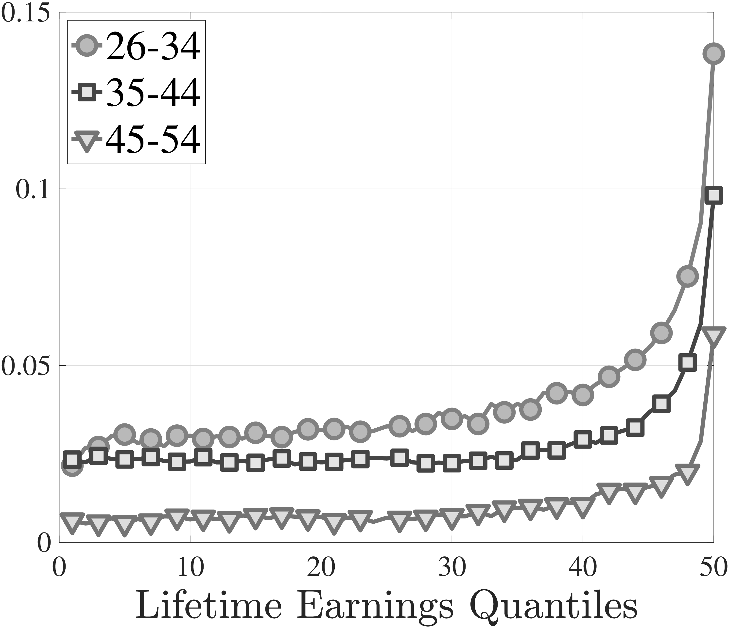
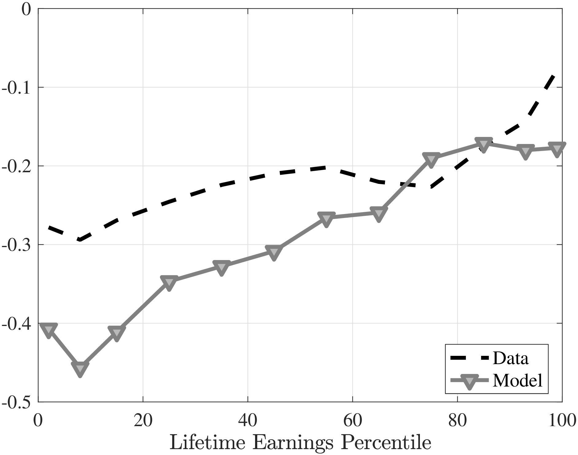
We compute lifetime earnings as the sum of individuals’ W-2 earnings from ages 25 to 55.6 This measure is then used to rank workers into 50 equally sized quantiles, \(LE_{j}\) for \(j=1,\ldots,50\). Individuals around the 90th percentile (\(LE_{45}\)) earn 3.7 times as much as those around the 10th percentile (\(LE_{5}\)) (see Figure 1a and Table A.2). This inequality is roughly half the annual earnings inequality, for which the ratio of the 90th percentile to the 10th percentile hovered around 8 throughout our sample period (Guvenen et al. (2014b)). Inequality is more pronounced at the top, with \(LE_{50}\) earning almost 4 times as much as \(LE_{45}\) versus \(LE_{5}\) earning almost twice as much as \(LE_{1}\).
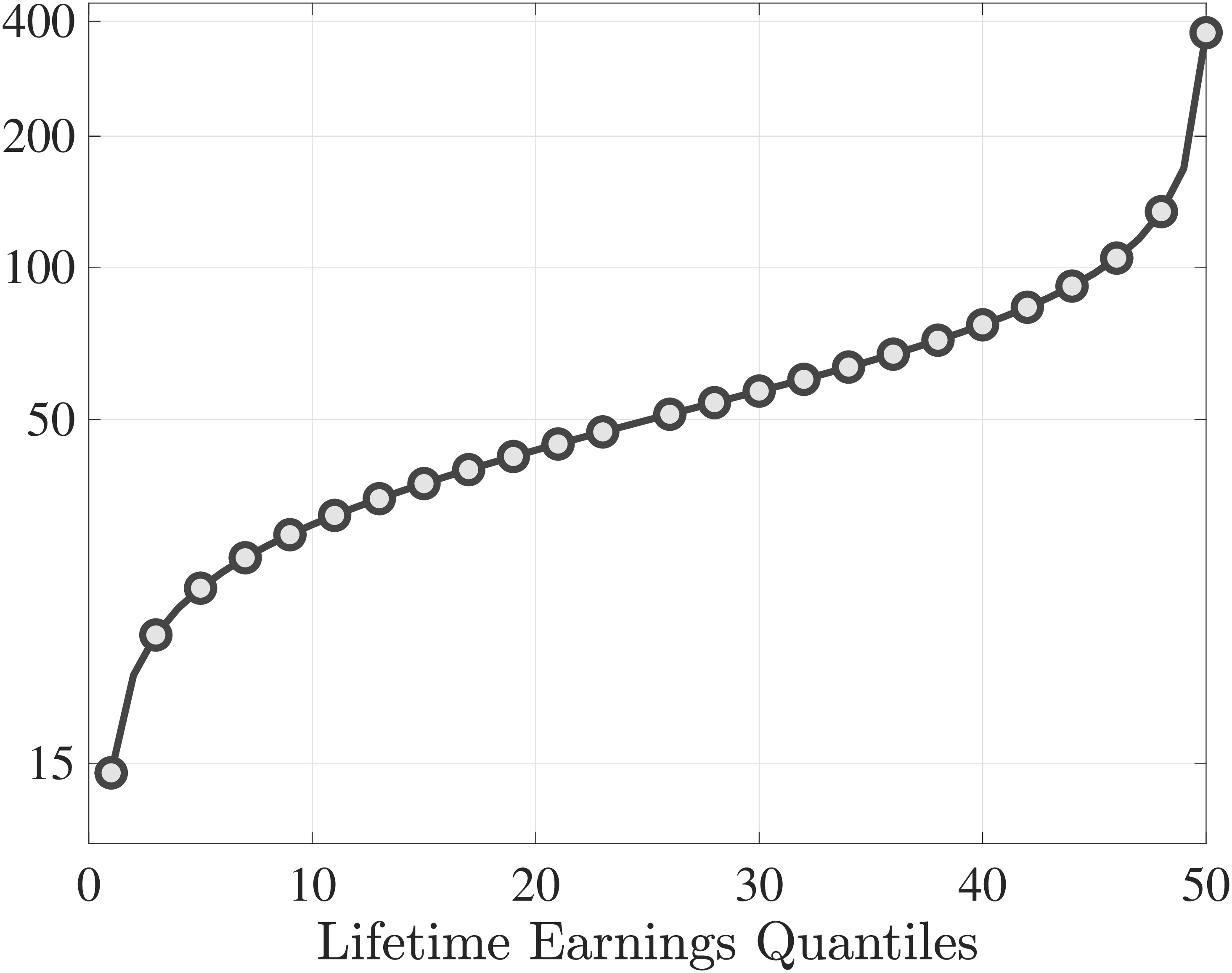
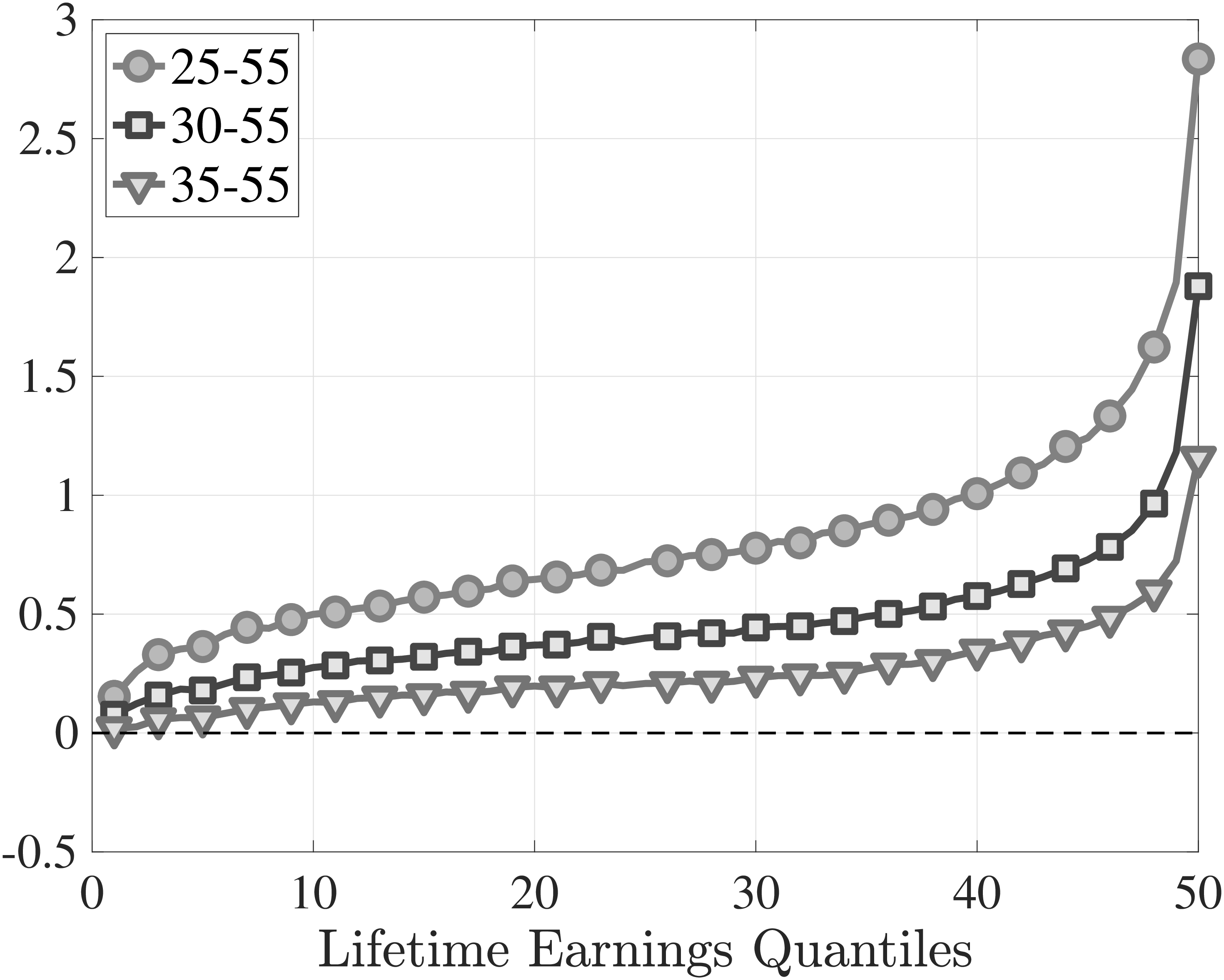
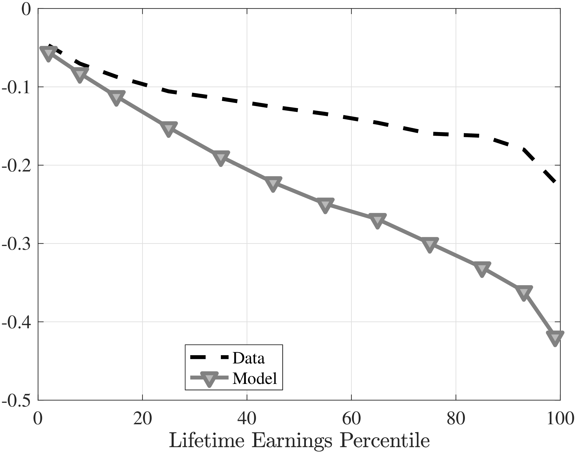
Notes: The left panel shows the average annual earnings over the life cycle by LE group. The right panel shows the log difference of average earnings \(\bar{Y}\) between age 55 and various ages over the LE distribution. For clarity we use one marker for every other LE quantile.
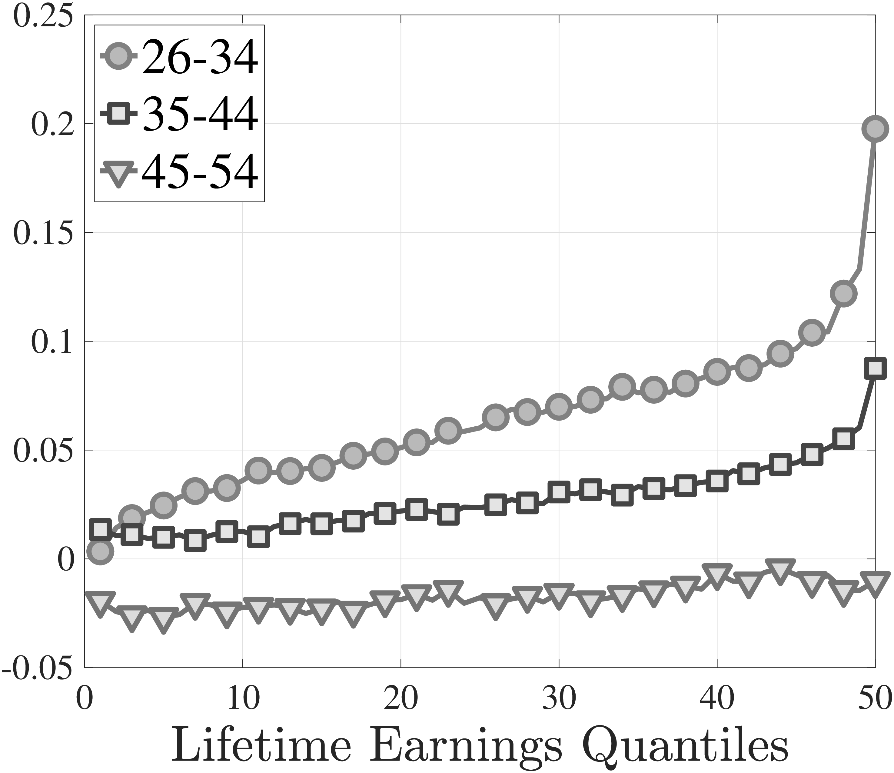
It is well known that in the U.S. differences in earnings growth over the life cycle are key for understanding the inequality in lifetime earnings (see, for example, Huggett et al. (2011) and Kaplan (2012)). To illustrate this point, Figure 1 shows the log growth of average earnings between different ages over the LE distribution; i.e., \(\log \overline{Y}_{h_{2},j}-\log \overline{Y}_{h_{1},j}\), where \(\overline{Y}_{h,j}\) is the average earnings of workers in LE \(j\) at age \(h\) (see Guvenen et al. (2021) for a similar figure from a broader sample). This growth measure allows us to include workers with zero earnings.7 Earnings growth is positively related to the level of lifetime earnings, which is not surprising, since, all else the same, one should expect the higher growth individuals to rank at the top of the distribution. However, the quantitative magnitudes are striking: The top LE earners (\(LE_{50}\)) see their earnings rise by more than 17-fold between the ages of 25 and 55, median workers experience a two-fold increase, whereas those at the bottom see little to no earnings growth (around 16%).8 As we quantify in Section 6, large differences in earnings growth make an unmistakable contribution to the lifetime earnings inequality.
Some of this steep rise in earnings growth at the top could simply be due to transition from school to employment in the labor market. For example, top LE individuals might be pursuing graduate degrees around earlier ages. While the lack of education data does not allow us to answer this question directly, Figure 1b plots earnings growth between the ages of 30 and 55 and 35 and 55 when schooling is unlikely to matter much. While the magnitudes change, we still find a steep profile of earnings growth with respect to LE, suggesting that low labor supply at age 25 is not the major driver of these patterns.
Top Earnings Inequality: A Brief Digression. As we discussed above, inequality is more pronounced at the top of the LE distribution. For example, the average annual earnings in the top 0.2% is over \(\$1,000,000\), compared to \(\$200,000\) for those around the 98th percentile. In fact, the right tail of the LE distribution follows a power law (Table A.2) with a a Pareto tail slope of –2.13 (Figure A.1). It is also already established that the population earnings distribution has Pareto tails (Piketty and Saez 2003; Atkinson et al. 2011). Importantly and interestingly, we find that this power law also holds in the cross-sectional distribution of earnings at each age (see Appendix A.2.1). Log density is linear in the tails at all ages and the slope gets closer to 1 in absolute value, which points to rising income concentration over the life cycle (Figures A.3 and A.4).
2.3 Career paths by lifetime earnings
A natural immediate question is: What accounts for the large differences in earnings growth? To this end, we investigate the differences in labor market experiences between LE groups. Earlier work has shown that job mobility is important for earnings growth over the life cycle (Topel and Ward (1992)). Therefore, we start by investigating how the number of (distinct) employers over the working life differs between LE groups.
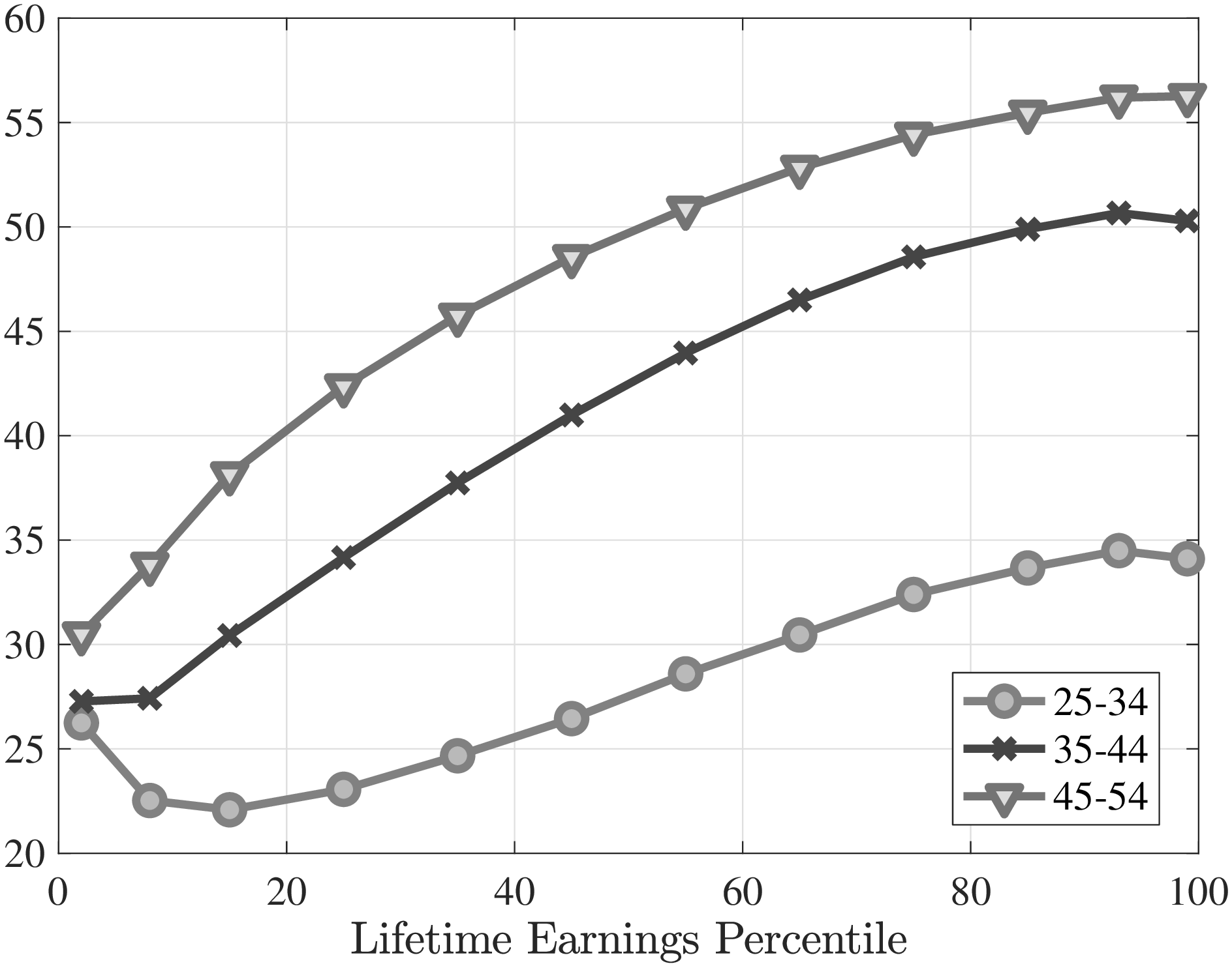
Individuals at the bottom of the LE distribution work for almost 5 different employers on average between ages 25 and 34, whereas the number of unique employers drops sharply to around 3 in the upper half of the LE distribution (Figure 2a). As workers age, job switching declines throughout the LE distribution but much more so in the upper half. While top workers work for around 1.5 different employers per decade after age 35, bottom workers still end up working for 3.5 employers on average, not much lower than the number of employers before age 35. At first glance, one might think that low LE individuals switch jobs very often and experience large earnings growth as a result. As we will see next, the nature of switches is very different across the LE groups.
We now document the average earnings growth across LE groups for workers who stay with the same employer and for those who change jobs. Given the annual frequency of the data, it is possible for job switchers to have more than one W-2 in a given year. Moreover, some workers may hold multiple jobs concurrently. These issues pose a challenge for a precise classification of job stayers and switchers. There is more than one plausible definition for a job stayer, and we opt for a conservative one. Specifically, we call a worker a job stayer between years \(t\) and \(t+1\) if i) he has income from the same employer in years \(t-1\), \(t\), \(t+1\), and \(t+2\); ii) his income in years \(t\) and \(t+1\) is above the minimum income threshold for that year; and iii) this employer accounts for at least 90% of his total labor income in years \(t\) and \(t+1\).9 This definition ensures that the main employer was the same firm in years \(t\) and \(t+1\). We label all other workers as job switchers. Note that according to this definition, switchers are a very heterogeneous group and consist of people who make direct job-to-job transitions, those who experience nonemployment, and those who come out of nonemployment. We return to this heterogeneity later.
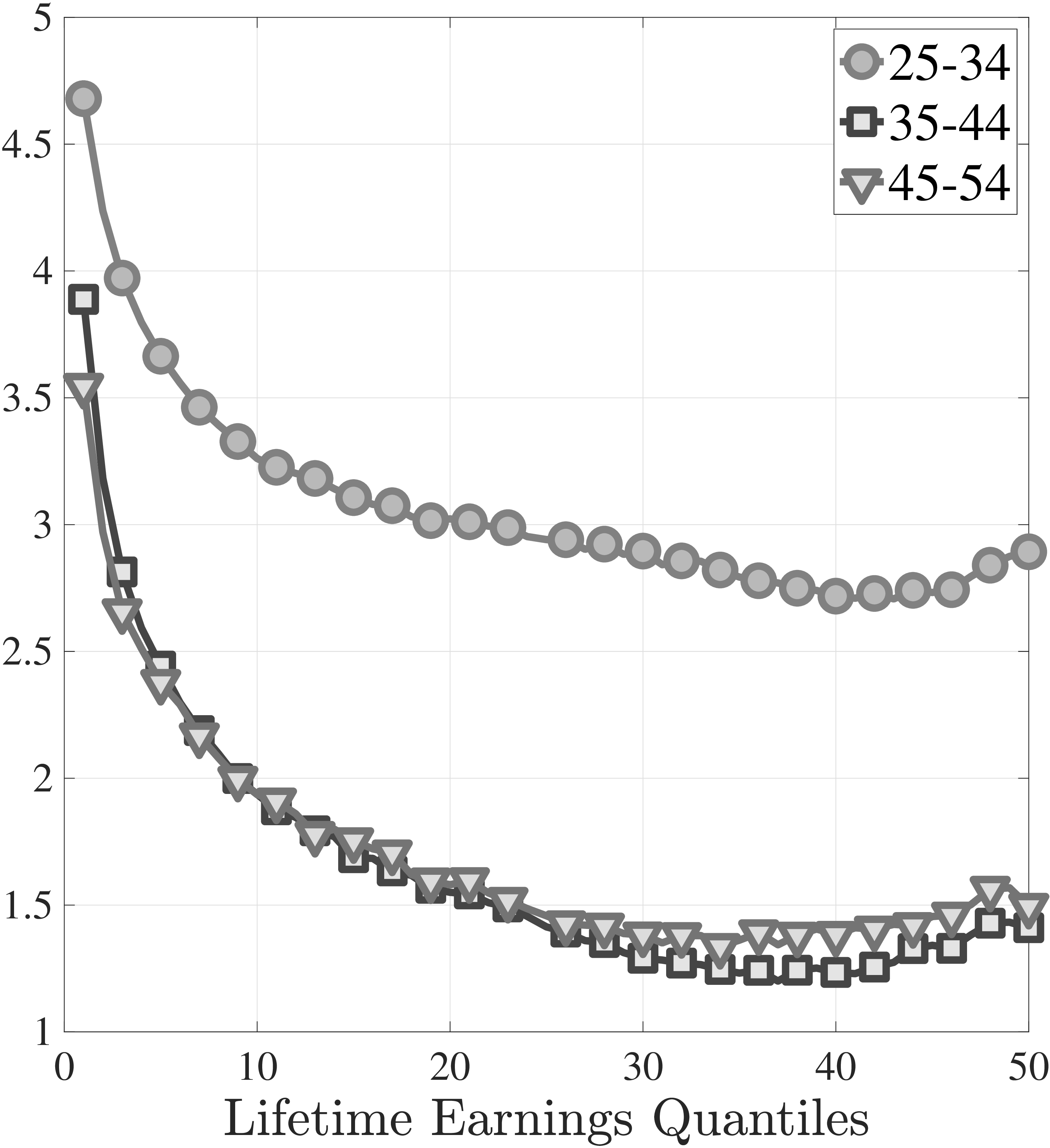
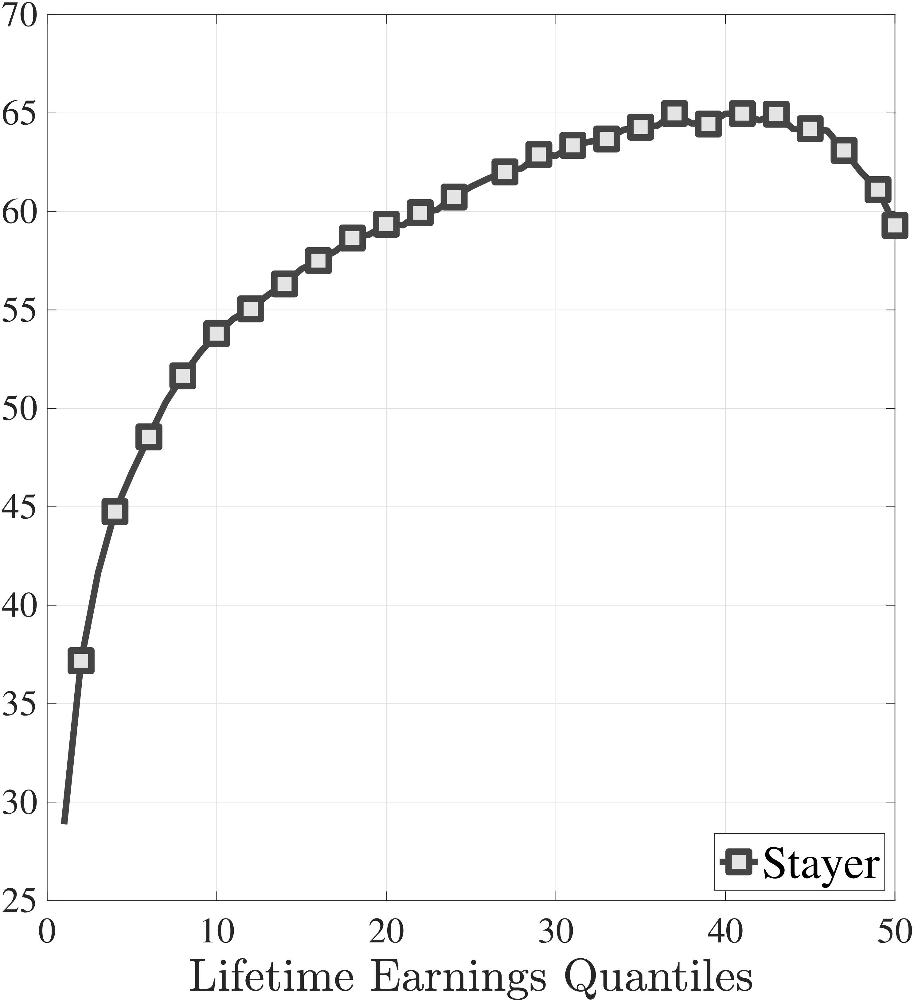
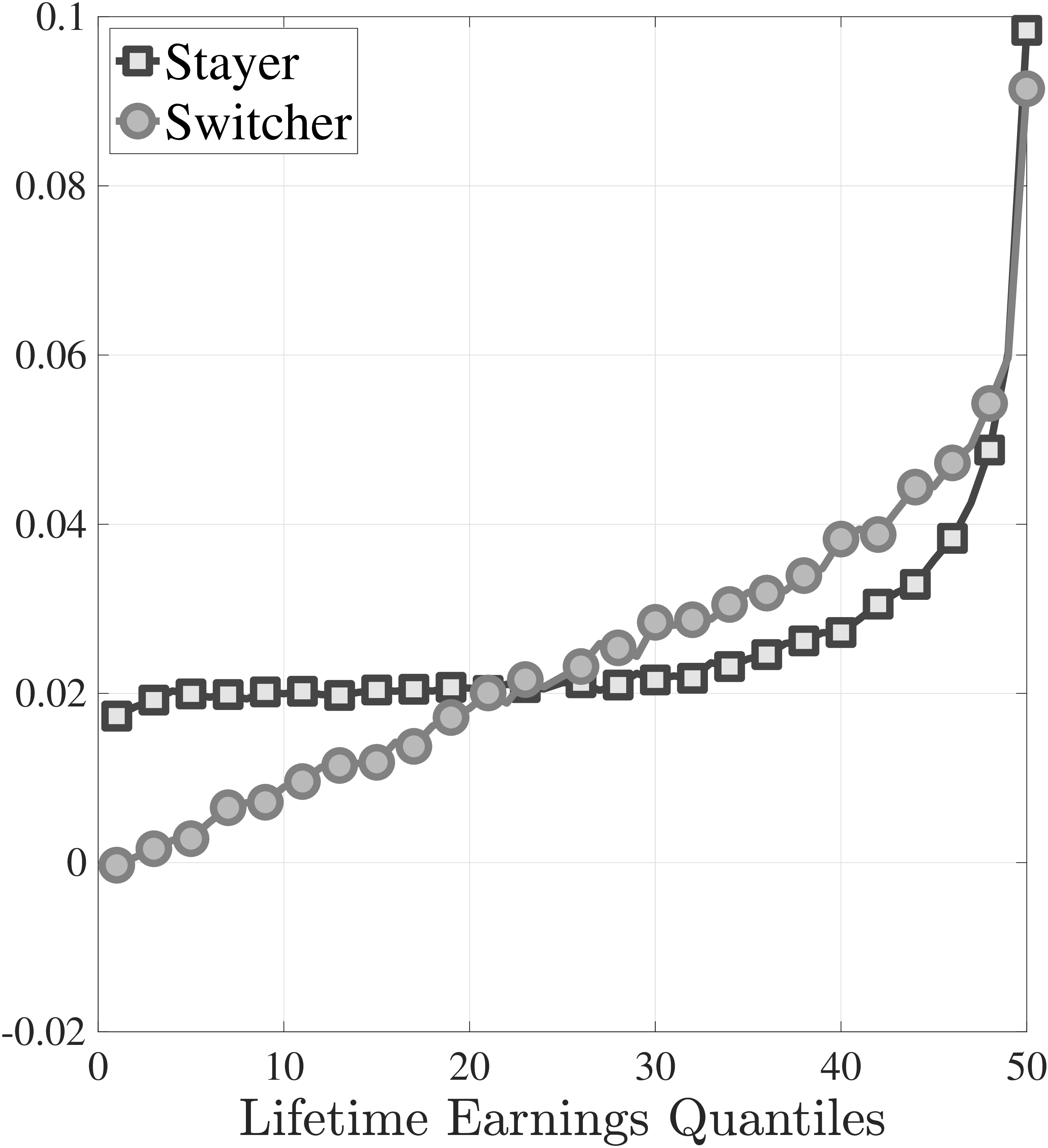
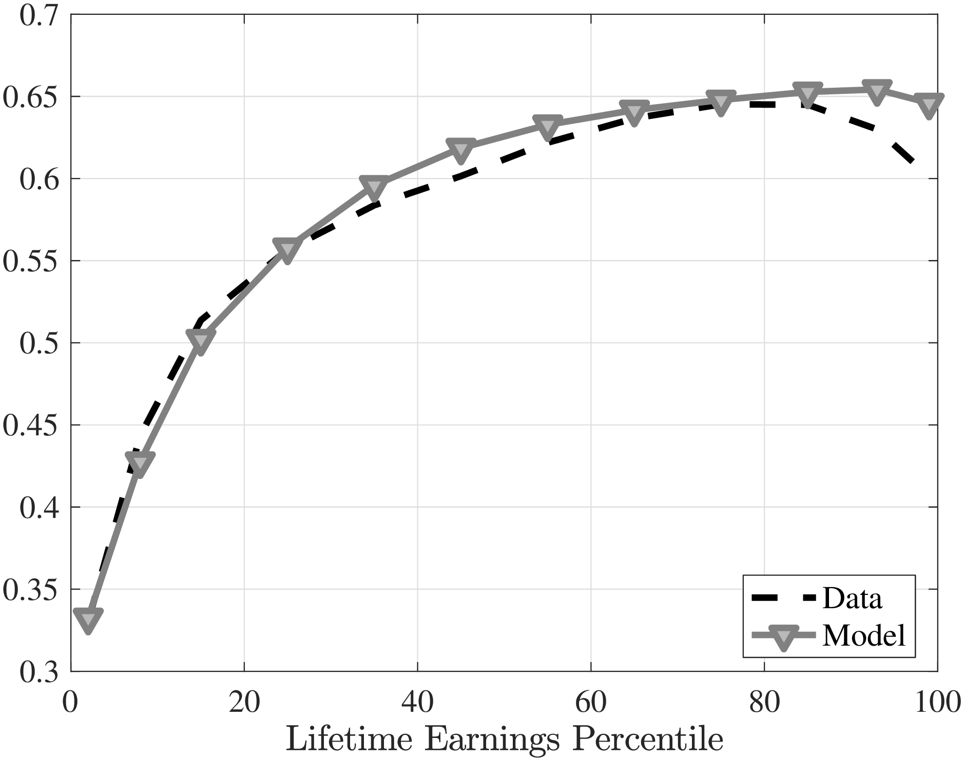
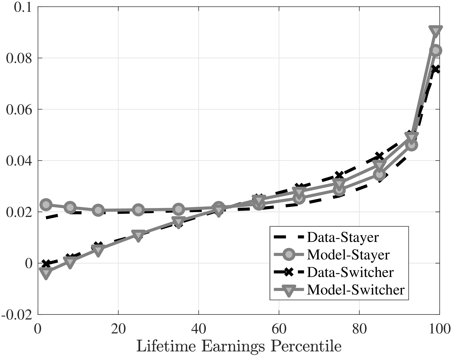
Notes: The left panel shows the number of distinct employers employers over the working life by LE. The middle panel shows the fraction of workers in each LE group who are job stayers according to our definition, calculated for each age and averaged over the working life. The right panel plots the log growth of average earnings \(\bar{Y}\) between \(t\) and \(t+1\) for job stayers and switchers separately by LE, again, averaged over \(t\) over the working life.
The middle panel of Figure 2 shows the fraction of job stayers within each LE group, averaged over the working life. Resonating with the large differences in the number of different jobs hold over the life cycle, bottom LE individuals stay with the same firm on average for 30% of their working life, compared to around 60% above the median.10
How much of an earnings growth does a worker experience when he stays with the same employer versus when he switches jobs? The answer differs widely across the LE distribution (Figure 2c). For job stayers log average earnings growth (between \(t\) and \(t+1\)) is surprisingly similar at around 2% in the bottom two thirds of the LE distribution. Whereas, average earnings growth for stayers increases sharply in the top LE tercile, reaching around 10% for \(LE_{50}\). Turning to job switchers, we find that average annual earnings growth is essentially zero at the bottom of the LE distribution and rises almost linearly to around 4% for \(LE_{45}\), after which it accelerates to 10% for the top LE individuals. This large heterogeneity indicates that the nature of job switches is very different throughout the LE distribution, which we will investigate shortly.11
These differences in earnings growth between job stayers and switchers are key for understanding the different forces behind the lifetime earnings growth over the LE distribution. For example, given the little heterogeneity among job stayers below the median LE, it is clear that the differences in lifetime earnings growth are due to the differences in the frequency and nature of job switches among these workers, suggesting large heterogeneity in job ladder risk for them. Whereas workers above the median LE are much more likely to stay with the same employer, therefore, large differences in earnings growth of job stayers should be the main culprit behind the lifetime earnings growth differences among them, suggesting large heterogeneity in returns to experience. Of course, wage growth of job stayers may also be determined by outside offers they do not accept or returns to experience is still a factor for earnings changes of job switchers. Thus, the exact decomposition of the importance of different economic forces requires a structural model estimated to match these salient features of the data (Section 3).
As we discussed before, job switchers are a very heterogeneous group as they include workers who switch jobs directly or due to a job loss (or a quit). The annual nature of the data does not allow us to separate these directly. Yet, we argue that the earnings growth distribution of switchers is informative about the nature of switches. For example, switchers who see their earnings decline by more than 25% have most likely experienced some nonemployment spell in \(t+1\). Thus, we classify such workers as “U-switchers,” and the remaining job switchers as “E-switchers.” The latter contains workers that make direct job switches as well as those coming out of nonemployment in \(t+1\).12
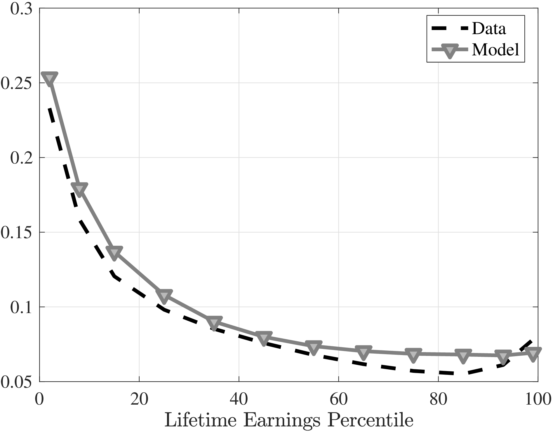
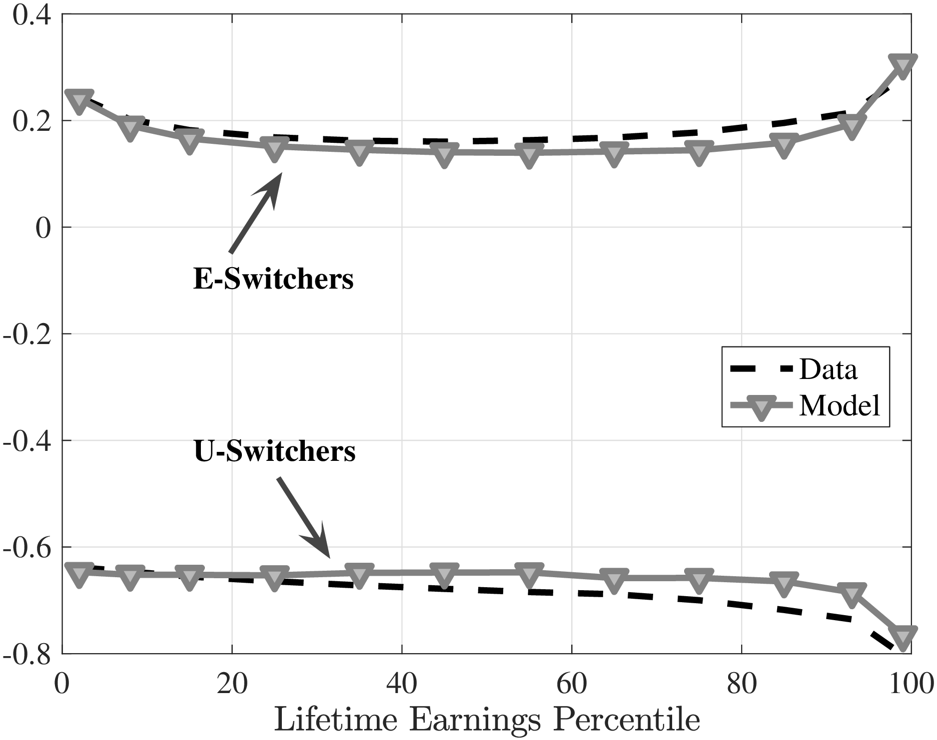
More than 35% of job switches are U-switches for bottom LE workers (Figure 3a). This share declines sharply over the LE distribution and reaches a low of 15% for \(LE_{40}\), before increasing to 20% for top LE workers. Thus, on average, higher LE individuals are more likely to make job switches involving earnings increases. Investigating the average earnings growth associated with each type of switch, we find large differences between E- and U-switches, but little variation across the LE distribution (except for the bottom and the top end). On average, an E-switch is associated with an earnings increase of larger than 15%, whereas a U-switch is associated with a decline of more than 60%.
The annual nature of our data limits the analysis of the earnings changes of job switchers.13 To investigate the role of annual aggregation in our results, we construct (normalized/average) earnings growth between the years when a worker is full-year employed in the same firm before and after the switch. Our substantive conclusions hold when we analyze this measure of earnings growth (Figure A.10). In addition, we investigate the monthly SIPP data, which allow us to construct direct measures of job loss (EU), job finding (UE), and job-to-job (EE) transition rates by income and age (see Appendix B for details). We find that low-income workers lose their jobs more often and the job finding rate is significantly lower for them (Figure B.1), therefore, they are more likely to make U-switches. In Section 5, we use these direct measures of quarterly job flow rates to quantitatively test our estimation results in an external validation exercise.
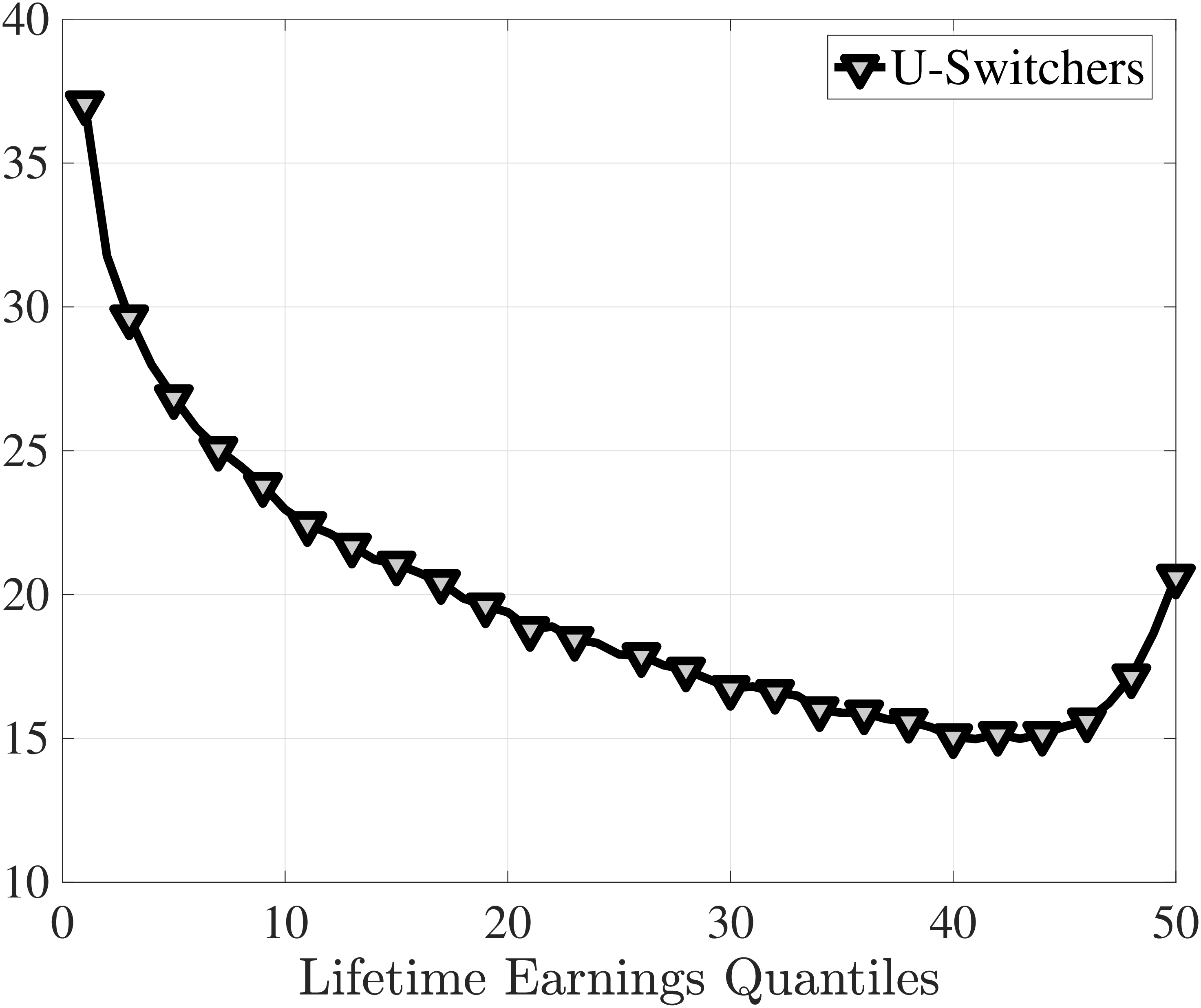
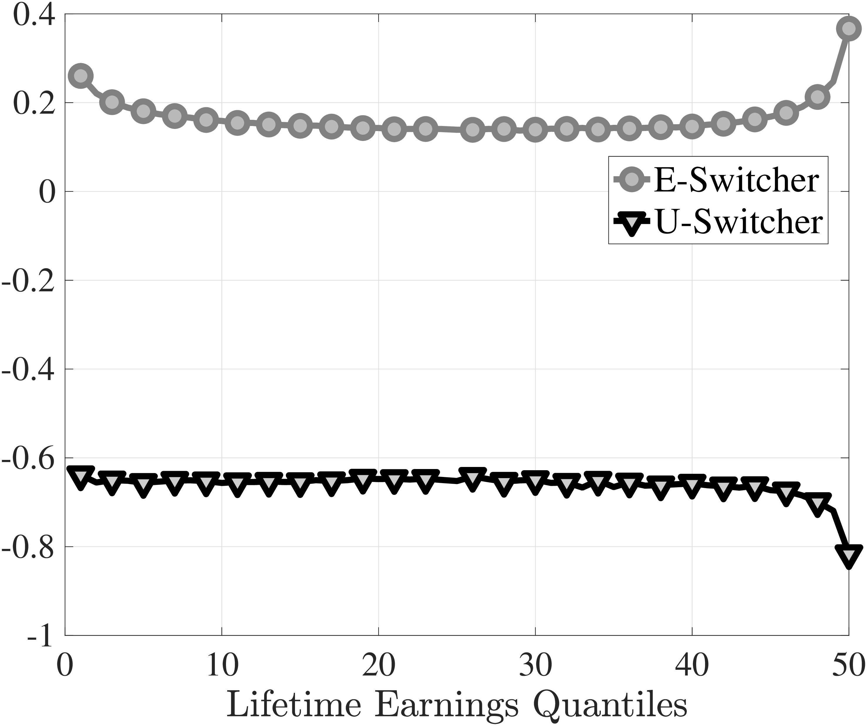
Notes: The left panel shows the share of U-switchers among job switchers averaged over the life cycle. The right panel plots the log growth of average earnings \(\bar{Y}\) between \(t\) and \(t+1\) for U- and E-switchers.
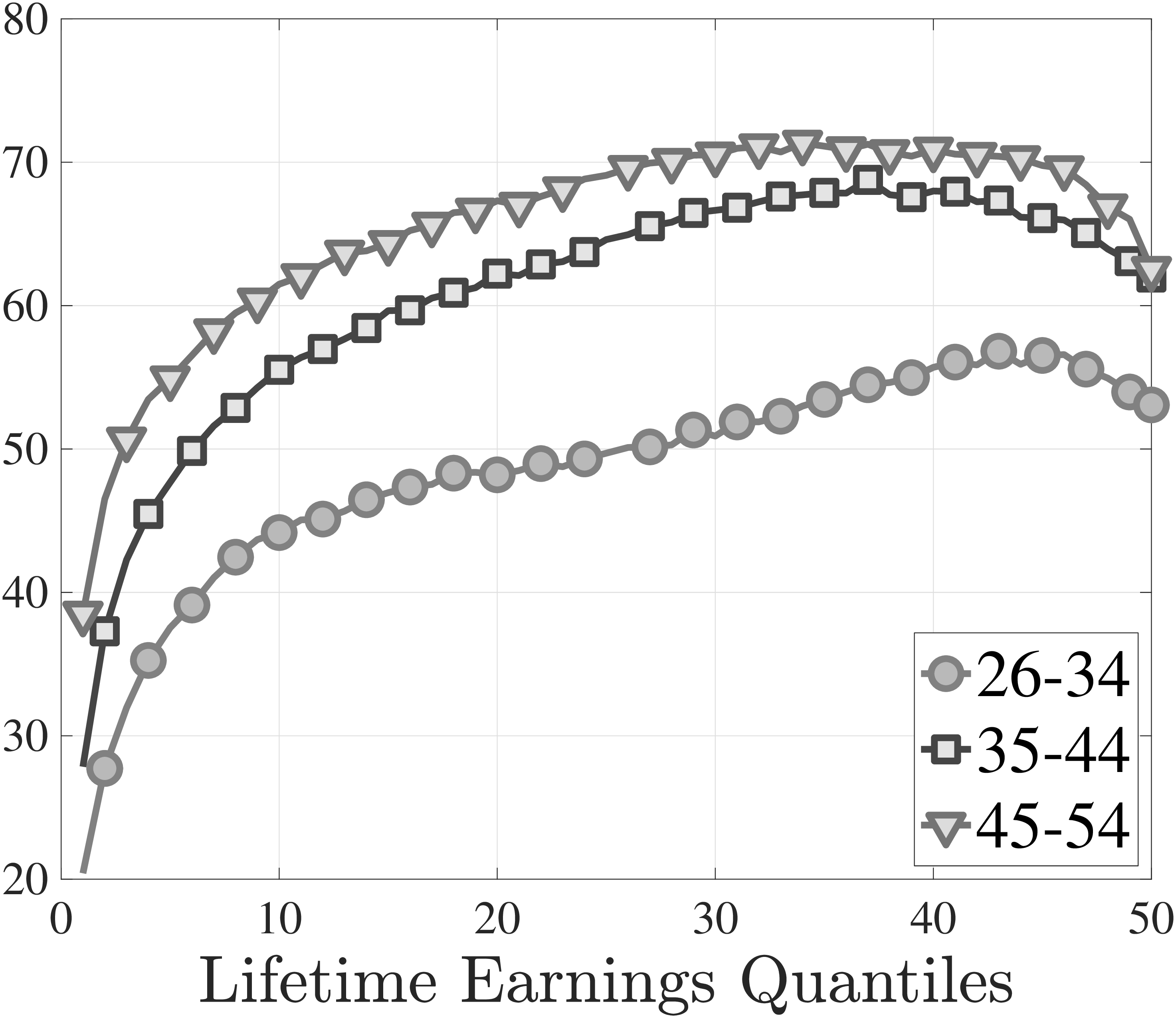
Life-cycle variation. Significant age variation in job switching and earnings growth rates has been extensively documented before (Topel and Ward (1992)). We contribute to this literature by investigating differences in these life-cycle profiles between income groups. Figure 4 plots the fraction of stayers and the earnings growth of job stayers and switchers for three stages of the working life over the LE distribution. The fraction of workers who stay with the same firm increases in a concave fashion over the life cycle for all LE groups. This increase is consistent with declining unemployment risk and job mobility documented before (Jung and Kuhn (2018)). Interestingly, the concavity is more pronounced above the median LE, resonating with larger decline in the number of distinct employers over the life cycle (Figure 2a).
Turning to the average earnings growth of job stayers, we find a flat profile below \(LE_{30}\) at all ages. Moreover, consistent with the existing literature, the rate of earnings growth declines with age. Similarly, the average earnings growth for job switchers also declines sharply over the life cycle, especially for higher LE workers, and becomes negative for oldest age group throughout the LE distribution (Figure 4c). Interestingly, being a job switcher or a stayer has limited effects on earnings growth of top LE workers before age 44, but it matters quite a bit for the oldest group. These individuals keep experiencing large earnings gains even after 44 when they stay with the same employer but their earnings decline if they switch jobs. In other words, in the top LE group earnings growth falls sharply for both job stayers and switchers over the life cycle but much more so for job switchers. This is because, first, U-switches become more likely among job switchers as the top LE workers get older. Second, and more importantly, average earnings growth for U-switches falls sharply for the oldest top LE workers (Figure A.8), which implies that unemployment spells become more costly for them. Our model is able to capture this feature of the data and we investigate it further in Section 5.
We have documented several facts regarding the careers of individuals who end up in different parts of the LE distribution. While these facts are useful for describing the various components of earnings growth heterogeneity, they do not suffice to provide an exact decomposition of the importance of the underlying economic forces or to separate ex-ante heterogeneity from ex-post luck. In what follows, we develop and estimate a structural model of wages and job turnover with heterogeneity in returns to experience and job ladder risk as well as ex-post productivity and job ladder shocks. In the end, this quantitative model will allow us to disentangle the various economic forces that shape the distribution of wage changes of job stayers and switchers.
3 Model
We build on Bagger et al. (2014) as it features a tractable framework to study the role of job search and learning on the job in generating wage growth.14 Despite endogenously generating some age variation in job mobility and earnings dynamics, this model falls short of capturing the magnitudes in the data. Thus, we incorporate stochastic aging to this framework à la Blanchard (1985). Furthermore, motivated by large negative earnings changes for job stayers, we also allow for recalls for unemployed workers by their last employers à la Fujita and Moscarini (2017). Next, we present our theoretical model and motivate each ingredient by linking them to specific empirical facts.
3.1 Environment
The economy is populated by heterogeneous workers and firms that produce a single consumption good sold in a competitive market. Workers can be employed or unemployed, and search for jobs in a frictional labor market, both on and off the job. They start life as young (\(y\)) and become old (\(o\)) with probability \(\gamma\). They have preferences with log per-period utility over consumption, and discount future periods at rate \(\rho\): U({c_{t}}{t=0}^{})={t=0}^{}()^{t}c_{t}. There is no inter-temporal savings technology that allows workers to smooth their consumption. This assumption along with the log preferences and log linear production function—which we introduce shortly—greatly simplifies computation.
Worker productivity. Each worker enters the labor market with no experience and accumulates human capital as he gains actual experience from employment. The human capital of worker \(i\) in period \(t\) is given by
\[ \begin{aligned} h_{it} & = & \tilde{h}_{it}+\epsilon _{it},\,\,\,\,\tilde{h}_{i0}=\alpha _{i}\\ \tilde{h}_{it} & = & \begin{cases} \tilde{h}_{it-1}-\varsigma & \text{if unemployed}\\ \tilde{h}_{it-1}+\beta _{i}+\zeta \left (\tau _{it}^{2}-(\tau _{it}-1)^{2}\right) & \text{if employed} \end{cases} \end{aligned} \]
Here, \(\tilde{h}_{it}\) denotes the deterministic component of human capital. Its level at \(t=0\), \(\tilde{h}_{i0}\), is determined by the worker’s type \(\alpha _{i}\), which reflects permanent heterogeneity in productivities due to differences in initial conditions such as innate ability, education, and labor market experience before \(t=0\). Human capital accumulates as the worker gains actual experience \(\tau _{it}\) through employment. Note that human capital is not specific to the firm, consistent with Gathmann and Schonberg (2010) who show labor market skills to be quite portable. Motivated by the large differences in average earnings growth for job stayers by LE, the rate of human capital accumulation has a worker-specific linear component \(\beta _{i}\), potentially correlated with \(\alpha _{i}\), and a common quadratic component \(\zeta\).15 In Huggett et al. (2011) individual-specific growth rates of human capital arise as a result of different investment choices due to the heterogeneity in productivities in the production of human capital. Our model captures this heterogeneity through exogenous differences in returns to experience. When a worker is unemployed, his human capital \(\tilde{h}_{it}\) depreciates at a constant rate \(\varsigma\).16 Finally, \(\epsilon _{it}\) is an idiosyncratic shock to worker productivity that captures the residual sources of variation in earnings not modeled in our framework, such as bonuses. Motivated by the large variation in the distribution of earnings changes for job stayers (Figure D.2), we assume that its distribution depends on worker type \(\alpha _{i}\) and age. We specify the process for \(\epsilon _{it}\) in Section 4 in detail.
Firm distribution and production technology. Productivity of a firm is constant over time and drawn from a distribution \(F(p)\) with a support of \(\left [\underline{p},\infty \right]\) common to all workers. A worker with human capital \(h_{it}\), who works for a firm with productivity \(p_{j(i,t)}\), produces a homogeneous good according to a log-linear production function, \(e^{y_{it}=p_{j(i,t)}+h_{it}}\).
3.1.1 Heterogeneity in search and matching
Unemployment risk. A job dissolves exogenously with probability \(\delta ^{a}(\alpha _{i})\), in which case the worker searches for a job. We model separation rates to be heterogeneous across workers of different types and ages. This heterogeneity is needed to capture the declining unemployment risk by the wage and age of workers discussed in Section 2.
Job finding rate. An unemployed worker of age \(a\in \{y,o\}\) with permanent ability \(\alpha _{i}\) meets a firm with probability \(\lambda _{0}^{a}(\alpha _{i})\), which captures ex-ante heterogeneity in job finding rates. This heterogeneity is motivated by our findings from the SSA and SIPP data and are potentially important for wage growth over the life cycle, as workers with a high job finding rate will work for more years, end up accumulating more human capital and, on average, work for more productive firms. To account for the sources of earnings growth, we explicitly model the differences in job finding rates. Furthermore, workers who are hit by separation shocks find a job immediately with probability \(\xi \lambda _{0}^{a}(\alpha _{i})\). As we discuss later, our model period is a quarter, and a nonnegligible fraction of laid-off workers find a job within three months (Abraham et al. (2016)). Moreover, there is evidence of transitions that look like direct job-to-job switches but are actually involuntary (Jolivet et al. (2006)). Thus, we allow for the possibility of finding a job within the same period.
Recalls. In the data, there are many job stayers who experience large declines in annual earnings. Strongly left-skewed idiosyncratic productivity shocks could in principle account for these large losses, in turn, we would have erroneously assigned a bigger role for ex-post productivity shocks especially for low-income workers (as opposed to their higher ex-ante unemployment risk). Instead, we allow for a recall option of unemployed workers by their last employers, which is fairly prevalent in the data (Fujita and Moscarini (2017)). Specifically, we assume that with probability \(\lambda _{r}\) the offers for unemployed workers come from their last employers. The recall option can alter the wages as it affects the value of a job to a worker. However, we assume that the option value of recall is not considered in the wage bargaining process.17 This assumption keeps the estimation computationally feasible as it allows us to derive the wage equation analytically.
Search on the job. While employed, workers search for better jobs and with probability \(\lambda _{1}^{a}(\alpha _{i})\) receive an outside offer from another employer, whose productivity is drawn from the distribution \(F(p)\), triggering a renegotiation between two firms that we explain below. As Figures 3a and B.1c have shown, workers differ in the types and rates of job switches. Our framework can generate qualitatively similar patterns without explicit differences in the contact rates: High-wage workers—employed on average by more productive firms—are less likely to get an offer that beats their current employer. This reduces their job-to-job transition rate even if they receive counteroffers at the same rate as low-wage workers. Similarly, as workers get older, they settle into higher paying jobs and are less likely to move. However, our estimation shows that this endogenous mechanism is insufficient to explain the quantitative differences in the data.
Timing of events. At the beginning of each period, the productivity shocks are drawn and workers’ human capital is updated according to equation 1. Next, output is produced and wages are paid. There is no inter-temporal savings device, so workers consume their wages. At the end of the period, search and matching shocks are realized: Unemployed workers who find jobs negotiate their wage, workers who receive an outside offer renegotiate their wages or switch employers, and employed workers that draw separation shocks become unemployed. They may find a job immediately or have to wait for the next period to search. Aging occurs stochastically at the end of the period with probability \(\gamma\) and is mutually exclusive from the labor market shocks.
3.2 Wage determination
We now briefly explain the bargaining protocol by focusing on the key equations and how the life-cycle structure affects them. See Appendix C for derivations.
Wages are specified as piece-rate contracts. In particular, if a worker with human capital \(h\) works for a firm of productivity \(p\) at a piece rate of \(R=e^{r}\leq 1,\) he receives a log wage \(w\) of \(w=r+p+h\). Here \(R\), the contractual piece rate, is determined endogenously. Upon meeting with a firm, the worker bargains over this piece rate \(R\), which is not updated until the worker meets with another firm.
We now describe how this piece rate is determined for workers with different labor market states. First, let’s define \(\mathbb{I}_{i}\equiv \{\alpha _{i},\beta _{i}\}\) as the vector of individual-specific state variables capturing ex-ante (fixed) heterogeneity. Note that as we discussed above, \(\mathbb{I}_{i}\) pins down the individual-specific worker flow rates as well as the firm distribution, i.e., \(\{\delta ^{y}(\alpha _{i}),\delta ^{o}(\alpha _{i}),\lambda _{0}^{y}(\alpha _{i}),\lambda _{0}^{o}(\alpha _{i}),\lambda _{1}^{y}(\alpha _{i}),\lambda _{1}^{o}(\alpha _{i})\}\). The value functions introduced below are individual specific and thus a function of \(\mathbb{I}_{i}\) in addition to other state variables.
Hires from unemployment. Let \(V_{0}^{a}\left (h;\mathbb{I}_{i}\right)\) and \(V^{a}\left (r,h,p;\mathbb{I}_{i}\right)\) denote the expected lifetime utility of an unemployed worker \(i\) with human capital \(h\) at age \(a\), and when he is employed at a firm with productivity \(p\) at piece rate \(e^{r},r<0\), respectively. We define \(V^{a}\left (r,h,p;\mathbb{I}_{i}\right)\) below and assume that the value of unemployment is equivalent to employment in the least productive firm of type \(p_{\min}\) extracting the entire match surplus, i.e., \(V_{0}^{a}\left (h;\mathbb{I}_{i}\right)=V^{a}\left (0,h,p_{\min};\mathbb{I}_{i}\right)\). This assumption—typical for this class of models and justified by the high empirical job acceptance rate of the unemployed (Van den Berg 1990)—implies that unemployed workers accept any job offer and simplifies the problem.
The wage bargaining protocol dictates that unemployed workers receive \(\theta\) share of the expected match surplus, where \(\theta\) captures the worker’s bargaining power.18 More specifically, the piece rate of a hire from unemployment, \(r_{0}\), solves
\[ \mathbb{E}V^{a}\left (r_{0},h',p;\mathbb{I}_{i}\right)=V_{0}^{a}\left (h;\mathbb{I}_{i}\right)+\theta \mathbb{E}\left [V^{a}\left (0,h',p;\mathbb{I}_{i}\right)-V_{0}^{a}\left (h;\mathbb{I}_{i}\right)\right]. \]
The worker’s surplus from the match is the increase in expected lifetime utility from unemployment to a state where he is paid his entire output (\(r=0\)). Thus, when an unemployed is hired, the firm offers a piece rate that increases his expected lifetime utility by \(\theta\) share of this surplus. In equation (2), the expectation is with respect to \(\epsilon _{t+1}\).
Poaching. When a worker is contacted by a firm with productivity \(p'\), the incumbent firm and the poacher compete. The more productive firm outbids the less productive one and hires the worker. We now discuss the wage that arises as a result of this competition.
There are several cases to consider. First, suppose that the poacher has higher productivity; \(p'>p\). Then, the poacher hires the worker by paying a piece rate \(r'\) that increases the worker’s value by \(\theta\)–share of the surplus generated by the match: \[ \mathbb{E}V^{a}\left (r',h',p';\mathbb{I}_{i}\right)=\mathbb{E}\left \{V^{a}\left (0,h',p;\mathbb{I}_{i}\right)+\theta \left [V^{a}\left (0,h',p';\mathbb{I}_{i}\right)-V^{a}\left (0,h',p;\mathbb{I}_{i}\right)\right]\right \}. \] Note that as Postel-Vinay and Robin (2002) have shown, job switches may result in workers accepting wage losses, as they anticipate faster wage growth in higher productivity firms. Wage losses upon job switches are a prominent feature of the data.
Second, let’s consider a case in which the poacher has lower productivity than the current employer. Bertrand competition implies that the incumbent firm retains the worker, possibly by adjusting the worker’s piece rate. This new piece rate offers the worker the maximum value he could attain working at firm \(p'\), i.e., the value associated with \(r=0\) (\(R=1\)), and a \(\theta\)–share of the additional surplus generated by the offer. In this case, the new piece rate \(r'\) solves the following equation: \[ \mathbb{E}V^{a}\left (r',h',p;\mathbb{I}_{i}\right)=\mathbb{E}\left \{V^{a}\left (0,h',p';\mathbb{I}_{i}\right)+\theta \left [V^{a}\left (0,h',p;\mathbb{I}_{i}\right)-V^{a}\left (0,h',p';\mathbb{I}_{i}\right)\right]\right \}. \] Note that in contrast to other models of on-the-job search such as Burdett and Mortensen (1998) and Hubmer (2018), this model generates potentially large and leptokurtic increases in wages for job stayers, which is prevalent in the data (Guvenen et al. (2021)).
In some cases, the productivity of the poacher may be so low that the new offer does not generate any additional surplus and therefore does not trigger a change in the piece rate. Then, the worker discards the offer. Let \(q^{a}(r,h,p;\mathbb{I}_{i})\) denote this threshold firm productivity such that offers from firms with \(p'\leq q^{a}(r,h,p;\mathbb{I}_{i})\) are discarded. \(q^{a}\) solves \[ \mathbb{E}V^{a}\left (r,h',p;\mathbb{I}_{i}\right)=\mathbb{E}\left \{V^{a}\left (0.h',q^{a};\mathbb{I}_{i}\right)+\theta \left [V^{a}\left (0,h',p;\mathbb{I}_{i}\right)-V^{a}\left (0,h',q^{a};\mathbb{I}_{i}\right)\right]\right \}. \]
4 Estimation
We now use this model to estimate the contributions of the heterogeneity in the worker flow rates and the ability to accumulate human capital to the differences in earnings growth over the life cycle. To this end, we first exogenously set four parameters: The quarterly discount rate \(\rho\) is set to 0.005 to match the annual rate of 2%; workers’ bargaining power \(\theta\) is set to 0.4 following Bagger et al. (2014); the quarterly aging probability \(\gamma\) is set to \(1/60\) so that a worker becomes old on average in 15 years; and the reallocation probability \(\xi\) is set to 0.4 following Abraham et al. (2016).
We estimate the remaining parameters using the simulated method of moments (SMM). We simulate quarterly data for 100,000 individuals and aggregate them to annual observations to create a matched employer-employee panel mimicking the SSA sample. Importantly, we subject the model to the same sample selection criteria in Section 2.1 and compute the model counterparts of targeted moments. Recall that our sample consists of workers between ages 25 and 55 (Section 2.1). However, estimation does not assume that workers start their careers at age 25. Instead, both in the data and the model we are agnostic about workers’ labor market experiences before age 25. Thus, previous labor market experience or time spent in school would show up as ex-ante heterogeneity in our estimation. In our simulations, each individual starts unemployed at the age of 23 and we discard the first two years to allow workers to find a job before age 25.
4.1 Targeted moments
We target five sets of moments. The first two are about the cross-sectional distribution of earnings changes for job stayers and switchers. The third and fourth have to do with the fraction of job stayers, E–switchers, and U–switchers and their average annual earnings growth, respectively. Finally, we target average earnings at age 25 by LE group. We choose to not target the heterogeneity in lifetime income growth. As we argue in the next section, the model is already identified using these five sets of moments.
Grouping workers. We condition each targeted moment on LE and age groups. Specifically, we calculate workers’ lifetime earnings as in Section 2 and rank them into 12 percentile groups: 1–4, 5–10, 11–20,…, 81–90, 91–96, 97–100. Furthermore, we group workers into three age groups: 25–34, 35–44, 45–54.
Cross-sectional moments of earnings growth. As documented in Guvenen et al. (2021), earnings changes are highly leptokurtic and left skewed. This shape of the earnings change distribution is broadly consistent with job ladder models: Most workers see little change but a small share experience a large swing due to unemployment, a job-to-job transition or an outside offer, which in turn may lead to a left-skewed and leptokurtic distribution. Based on these insights, we target the mean, standard deviation, skewness, and kurtosis of annual earnings changes for job stayers and switchers separately.19 We also condition workers based on their lifetime earnings because of large variation in these moments by income (Guvenen et al. (2021)).
An issue when computing growth rates is dealing with zero earnings. Recall that in our sample, we drop workers with two or more consecutive years of zero earnings. However, there are still observations with no income in a given year. We would like to keep them as they contain information about the importance of search frictions. For this purpose, we use the arc percent growth measure defined as \(2(Y_{t+1}-Y_{t})/(Y_{t+1}+Y_{t})\), where \(Y_{t}\) is annual earnings. Targeted cross-sectional moments are shown in Figure D.2.
Average income growth moments. Next, we target the fraction and average income growth of job stayers, E–switchers, and U–switchers by three age and 12 LE groups. The details of how these moments are constructed are discussed in Section 2.3. Figures D.1 and D.3 show these moments by age and the targeted LE groups.
Average earnings at age 25. Finally, we target the average earnings by LE group at age 25. This moment of the data is shown in Figure D.4.
4.2 Identification
Below we provide an informal discussion of identification of our model. We acknowledge that all parameters are determined jointly within the SMM estimation as most parameters affect more than one aspect of the data. In this section, our goal is to show that each feature of the model has a pronounced effect on at least one unique moment targeted in the estimation. Namely, there is at least one unique feature of the data that informs each ingredient of the model. This identification discussion also justifies the selected targeted moments presented in the previous section.20
Ex-ante worker productivity (\(\alpha,\beta\)). The concave average life-cycle profile of earnings growth is informative about the average experience profile of worker productivity, driven in the model by the mean of the joint (\(\alpha,\beta\)) distribution and the common quadratic term \(\zeta\). The differences in the initial earnings levels of LE groups and their stayer earnings growth (Figure 2c) help us pin down the variance-covariance matrix of the joint distribution of \(\alpha\) and \(\beta\). Note that the distribution of firm productivities also has a first-order effect on the initial earnings dispersion as well as on the earnings growth of job stayers through outside offers. As we discuss next, we use other features of the data to identify the distribution of firm productivities.
Firm productivity distribution. In the estimation of job ladder models, identifying the distribution of firm productivities is a key challenge. There are several approaches to estimate this distribution using matched employer-employee data.21 For example, Postel-Vinay and Robin (2002), Cahuc et al. (2006) and Bagger et al. (2014) use data on firms’ value added or profitability to back out the firm distribution. We cannot implement this method as our dataset doesn’t contain any direct information on value added or profitability. Barlevy (2008) shows that under appropriate conditions the wage gains of job switchers could identify the offer distribution nonparametrically, even in the presence of unobserved worker heterogeneity. Bagger and Lentz (2014) use poaching patterns between firms to rank firms with respect to their productivity. More recently, Bonhomme et al. (2017) uses k-means clustering to classify firms into discrete groups.
The key insight for our approach of identifying the firm productivity distribution relies on differences in earnings growth between job stayers and switchers, with stayer growth exhibiting relatively little heterogeneity at the bottom two thirds of the LE distribution and switchers showing much larger differences throughout the LE distribution (Figure 2c). If there was no job ladder to be climbed (i.e., a degenerate firm distribution), then the average earnings growth of switchers and stayers would look very similar (especially in the upper half of the LE distribution) as they would both be mainly driven by the differences in \(\beta\). Job ladder dynamics through the shape of the firm distribution, on the other hand, help the model generate a different profile of earnings growth for stayers and switchers. We confirm this insight by investigating the sensitivity of \(\psi _{f}\) to switcher earnings growth moments à la Andrews et al. (2017) (see Appendix D.2).
Heterogeneity in worker flow rates (\(\delta ^{a}(\alpha),\lambda _{0}^{a}(\alpha),\lambda _{1}^{a}(\alpha),\lambda _{r}\)). Our strategy relies on identifying these flow rates separately for each LE and age group and then linking the LE groups to ex-ante worker type \(\alpha\). U–switches, those that involve a larger than 25% earnings loss (Figure 3b), are intimately linked to the job loss rate \(\delta\). Moreover, their frequency is not affected by the rate of job-to-job transitions, because such transitions result in either wage increases or wage losses smaller than 25%, and are therefore counted among E-switches.22 Turning to the job finding rate \(\lambda _{0}\), this rate determines how long a given unemployment spell lasts. Therefore, it has a pronounced effect on the average earnings loss of U–switchers along with the possible wage decline associated with falling off the job ladder. The latter is determined by the shape of the firm distribution, whose empirical underpinning is discussed above. Finally, the stayer probability is given by a combination of the job loss rate \(\delta\) and the offer arrival rate for the employed \(\lambda _{1}\) as well as the recall rate \(\lambda _{r}\). The key feature that identifies the recall rate is the left skewness of earnings growth for job stayers. In the model, stayer growth distribution is dramatically right skewed in the absence of recalls. Having already identified \(\delta\) and \(\lambda _{r}\), stayer probability can now be used to pin down \(\lambda _{1}\).
Idiosyncratic shocks (\(\epsilon\)). They are residuals of earnings growth not explained by the structural features of the model. Our simulations show that the endogenous mechanisms can explain well the earnings dynamics of job switchers. Thus, we use the higher-order moments of earnings changes for job stayers to identify the idiosyncratic risk.
Age dependence in parameters. Targeted moments identifying the flow rates and the distribution of idiosyncratic shocks have strong age variation in the data (see Section 2), which we exploit to identify the age dependence in these parameters.
4.3 Estimation methodology
In this section we first explain the functional form assumptions concerning the worker and firm distributions as well as the flow rates. While our identification strategy does not require specific functional forms, these assumptions allow us to have more statistical power and keep the estimation computationally feasible. Next, we describe the SMM objective function along with the computational method used for estimation.
Functional forms. The worker fixed-effect \(\alpha\) is normally distributed with mean \(\mu _{\alpha}\) and standard deviation \(\sigma _{\alpha}\). \(\beta\) is Pareto distributed with shape and scale parameters \(\chi _{w}\) and \(\psi _{w}\), respectively, and is correlated with \(\alpha\) by the coefficient \(\rho _{\alpha \beta}\). We also estimated a version of our model with Gaussian \(\beta\) and have found that a fat-tailed distribution such as Pareto helps the model better match the very large earnings growth of top LE groups relative to the median and the relatively smaller differences between the median and the bottom LE groups.23 We revisit this choice later in the context of estimation results in Section 5. Firm productivity is also assumed to be Pareto distributed with shape and scale parameters \(\chi _{f}\) and \(\psi _{f}\), respectively.24 We normalize the scale parameter \(\psi _{f}\) to 1, as one cannot separately identify \(\psi _{f}\) and the mean of the \(\alpha\) distribution.
We model the heterogeneity in worker flow rates as a function of worker type \(\alpha\) and age. In particular, we use a cubic spline to model unemployment risk, the job finding rate, and the contact rate as a function of \(\alpha _{i}-\mu _{\alpha}\) for each age group. We experimented with the number of points for each flow rate and concluded that three points for each age group was flexible enough for job finding and contact rates, whereas unemployment risk required 5 points for each age to fit the heterogeneity in the data.
Finally, we assume that the i.i.d idiosyncratic shocks hit only job stayers once a year with some probability \(\pi (\alpha)\) (because endogenous mechanisms can explain well the earnings dynamics of job switchers). Innovations are normally distributed with standard deviation \(\sigma _{\epsilon}\) and \(\pi (\alpha)\) is modeled as a cubic spline separately for each age group.25
SMM objective function. Let \(d_{n}\) for \(n=1,...,N\) denote a generic empirical moment, and let \(m_{n}(\theta)\) be the corresponding model moment that is simulated for a given vector of model parameters, \(\theta\). The scales of the moments vary largely, thus we measure the distance between the data and the simulated moments by arc percentage deviation, \(F_{n}(\theta)=2\times \frac{m_{n}(\theta)-d_{n}}{m_{n}(\theta)+d_{n}}\). Our SMM estimator is then defined by \(\hat{\theta}=\arg \min _{\theta}\boldsymbol{F}(\theta)'W\boldsymbol{F}(\theta)\), where \(\boldsymbol{F}(\theta)=\left [F_{1}(\theta),...,F_{N}(\theta)\right]^{T}\). The weighting matrix \(W\) reflects our beliefs on the importance of each set of moments in identifying the economic forces behind earnings growth.26 We target a total of 380 moments to estimate 41 parameters.
Numerical method for estimation. We employ a multistart global optimization algorithm available by Guvenen and Ozkan (2021). In particular, we generate 15,000 uniform Sobol (quasi-random) points, compute the objective value for each of these, and select the best 1,000 (ranked by the objective value), each of which is used as an initial guess for the local minimization stage. This stage is performed with a mixture of Nelder-Mead’s downhill simplex algorithm and the DFNLS algorithm of Zhang et al. (2010). In the end, we pick the best parameter estimates out of 1,000 local minima.
5 Estimation Results
5.1 Parameter estimates
We first discuss the key parameter estimates by relating them to the moments that inform them the most. The full set of estimates are presented in Appendix D.
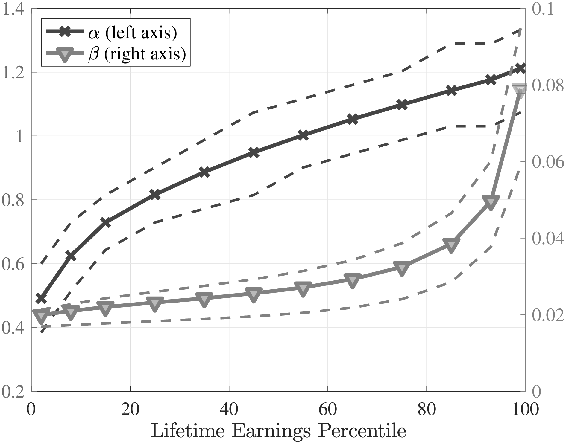
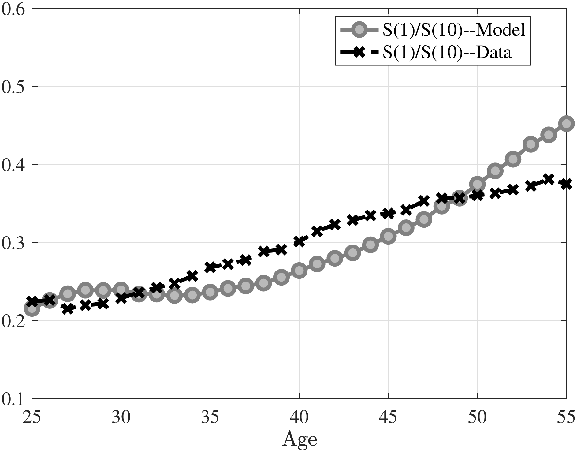
Notes: The left panel shows the mean of the distributions of \(\alpha\) and \(\beta\) by LE groups. Both distributions have been demeaned to have mean zero in the overall distribution. The right panel shows the ratio of incomes earned by the top 1% earners \((S(1))\) relative to the top 10% earners (\(S(10\))).
Distribution of \(\alpha\) and \(\beta\). We start by investigating the heterogeneity in permanent ability \(\alpha _{i}\) and the returns to experience \(\beta _{i}\) (Figure 5a). \(\alpha\) increases almost linearly throughout the LE distribution. Top LE individuals have an \(\alpha\) that is more than 60 log points larger than that of those at the bottom. Moreover, there is a sizable variation within each LE group. The interquartile range (dashed lines in Figure 5a) is around 10 log points. Together with this, the standard deviation of \(\alpha\) in the entire population is \(0.25\). Return to experience, \(\beta\), also increases with LE—not surprising given its positive correlation with \(\alpha\) of \(\rho _{\alpha \beta}=0.44\)—however with a different shape: \(\beta\) is relatively flatter in the bottom two-thirds and increases steeply towards the top.27 Clearly, this variation of \(\beta\) by LE is dictated largely by the shape of its distribution, which is assumed to be Pareto to match the average earnings growth differences of job stayers (Figure 2c).
The Pareto distributed \(\beta\), along with a Pareto firm productivity distribution, implies that earnings distribution exhibits power law throughout the life cycle as in the data (Figure A.2). While not targeted in the estimation, the model tracks the relative earnings share of the top 1% in the top 10% fairly well from age 25 to 50, after which the relative share in the model increases faster, driven by the growing importance of the return heterogeneity (Figure 5b). Note that typical models of top income inequality deliver a Pareto distribution through the accumulation of random returns over long periods of time, therefore, log income is exponentially distributed in the entire population (e.g., see Gabaix et al. (2016); Jones and Kim (2018)). However, the distribution of log income within each age is Gaussian in the random growth setting or in a process with normally distributed “growth types” (see Guvenen et al. (2014a) who also argue that several other features of the MEF data are not consistent with this mechanism of top inequality).
Human capital depreciation. We estimate human capital depreciation to be around \(1.5\%\) on a quarterly basis, larger in magnitude than estimated in Jarosch (2015) using German data. This is not the only channel in our model that contributes to scars from unemployment, which are large and persistent (Von Wachter et al. (2009), Krolikowski 2017). An unemployed worker also loses search capital, negotiation rents as well as the forgone opportunity of accumulating experience.
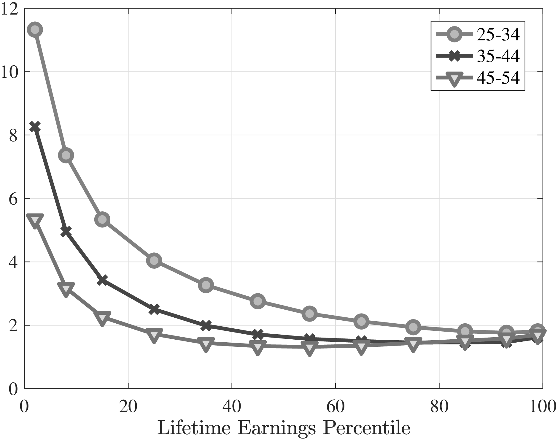
Heterogeneity in flow rates. Figure 6 plots in three panels how the quarterly unemployment risk, the job finding rate, and the contact rate vary with calendar age and LE groups.28 Unemployment risk, \(\delta ^{a}(\alpha)\), declines sharply with lifetime earnings up to median LE and is essentially flat for individuals above the median (Figure 6a). The job loss rate for bottom-LE workers is around four times as high as that for above the median workers. For example, for the youngest age group it declines from around 12% for the bottom earners to less than 3% for median workers. Consistent with previous work, we find the unemployment risk to be significantly higher for younger workers (see Shimer (1998) and Jung and Kuhn 2018). However, the life-cycle variation in unemployment risk is dwarfed by the differences between income groups, which we also observe in the SIPP data (Figure B.1).29 For example, for median workers job loss rate declines from around 3% to less than 2% over the life cycle. Furthermore, even though they see a significant decline in their job loss rate, bottom-LE workers never achieve the job stability above-median workers enjoy.
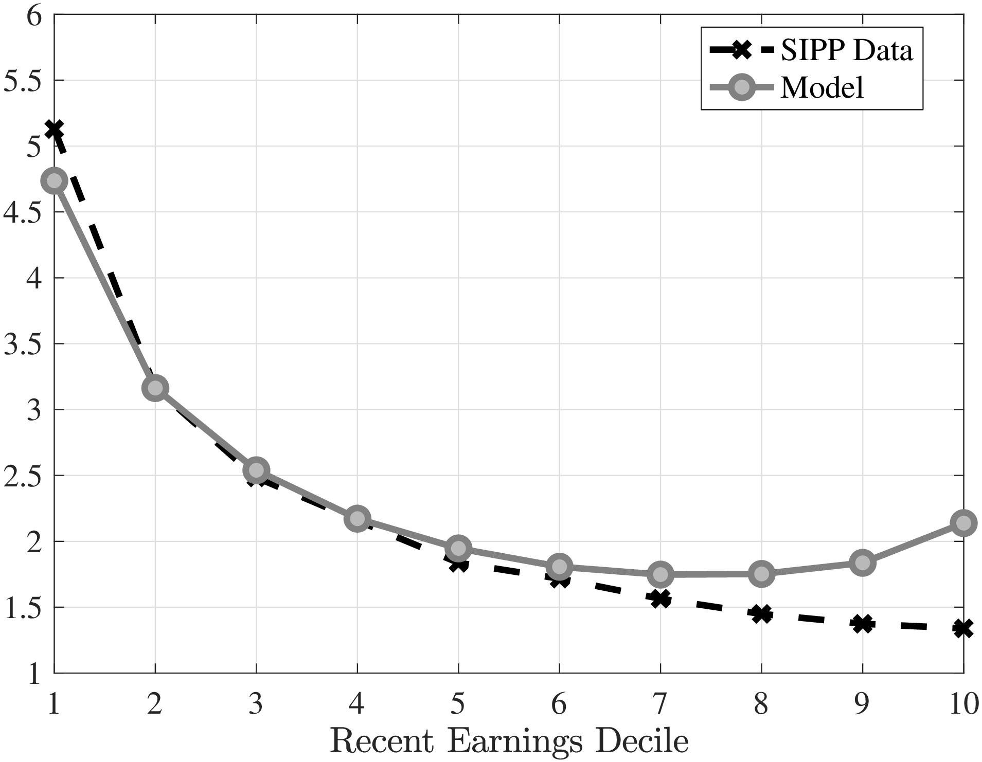
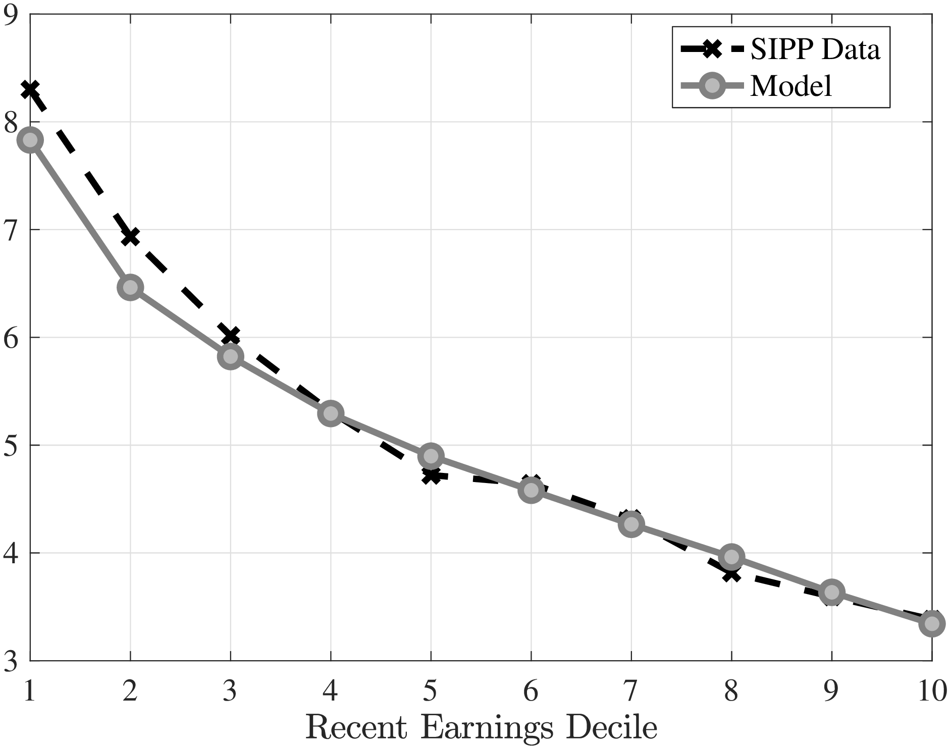
Given the annual nature of the SSA data, we cannot directly test these estimates. Instead, we investigate how the model fits the evidence on heterogeneity in job flow rates from the high-frequency SIPP data. SIPP contains monthly observations in overlapping panels with length between 2.5 and 4 years.We select a sample of males (ages 25–55) with strong labor force attachment (see details in Appendix B). We rank them into 10 equally sized deciles within each age group (25–34, 35–44 and 45–55) based on their recent earnings (RE) over the past three years. Next, we compute the EU, UE, and EE transition rates for each group over the next four months. We also follow the exact same sample construction in the model-generated data. Figure 6b shows how the unemployment risk varies with recent earnings in the SIPP data averaged over the life cycle along with its model counterpart (for separate age groups see Figure D.7). While not explicitly targeted in the estimation, the model captures remarkably well the extent of variation in the data, except for the top decile, where there is a slight uptick in the model-based EU rate but not in its empirical counterpart.
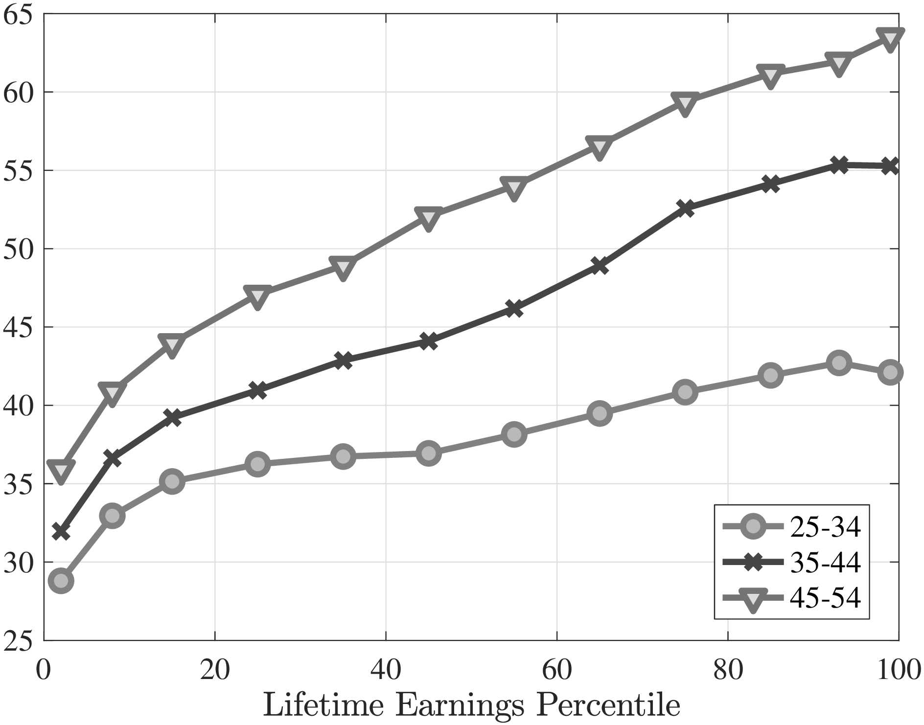
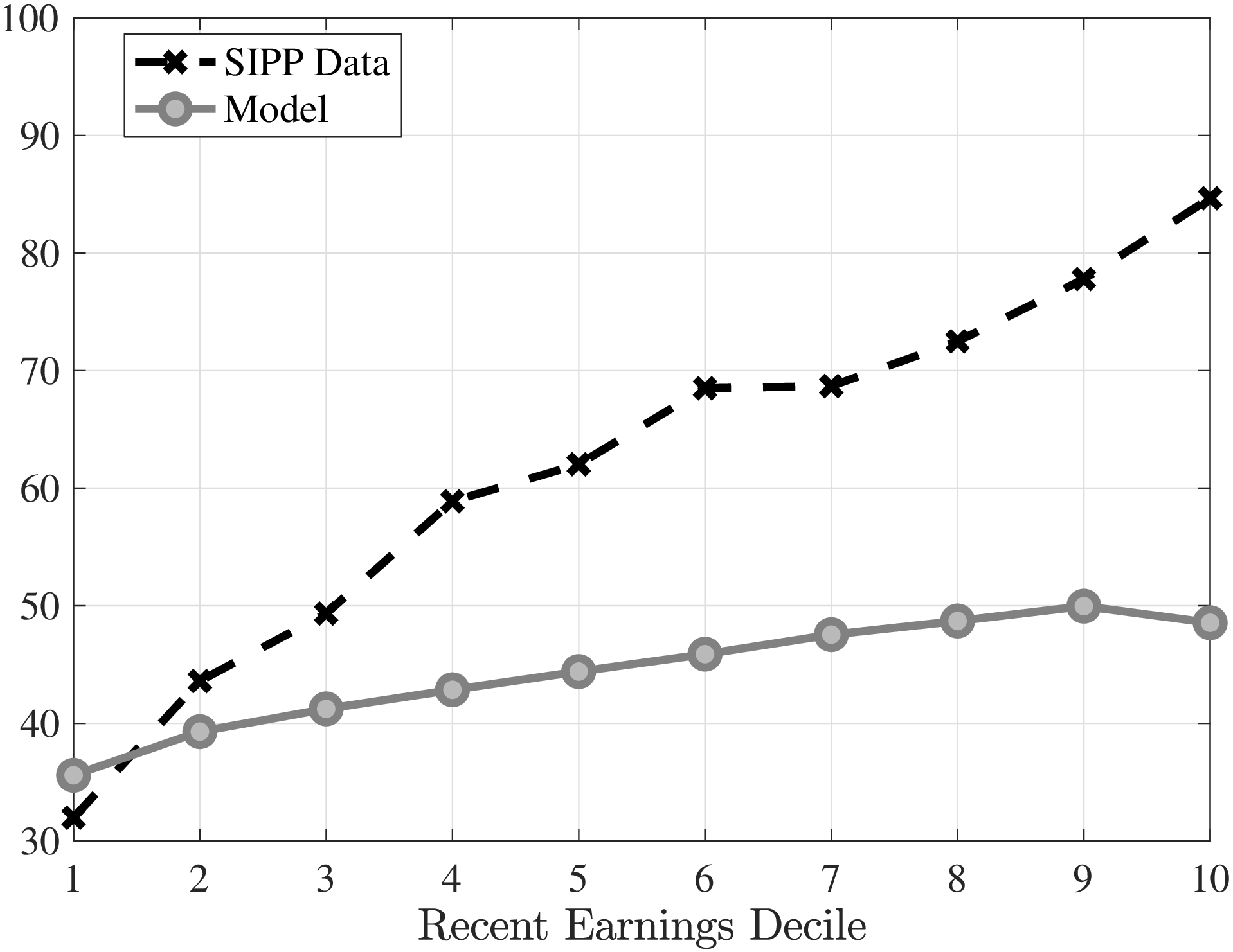
We estimate the job finding rate to be increasing with LE and age (Figure 6c). For example the quarterly job finding rate increases from around 30% at the bottom for workers ages 25–34 to above 60% at the top for workers ages 45–54. These estimates imply that the youngest bottom LE workers stay unemployed for around 3 quarters, compared to less than 2 quarters for the oldest top LE individuals.30 Coupled with an especially high unemployment risk for low LE workers, these estimates imply large differences in actual experience over the life cycle (Figure 9b). In particular, quarters worked over the working life range from 90 for low LE individuals to 120 at the top, which then have implications for earnings growth differences that we discuss later. The increasing job finding rate across the income distribution is qualitatively consistent with the evidence from the SIPP (Figure 6d), however, it does not increase as much as the data.31 There is also almost no age variation in the data in job finding rates, whereas the model estimates are systematically higher for older workers.
We estimate that 12.5% of unemployed workers are recalled back by their last employer (\(\lambda _{r}=0.125\)). This recall probability is lower than the 40% measured in Fujita and Moscarini (2017) for the US. They measure recalls directly using survey data from the SIPP, whereas we infer them indirectly to match the left tail of the earnings growth distribution of job stayers.
Turning to the contact rate for employed workers, we find this to be increasing with lifetime earnings and age, with a range between 25% and 55% (Figure 6e).32 While the increasing contact rate with LE and age seems contradicting with a declining job-to-job transition rate by RE and age in the SIPP data, the model actually captures both of these patterns well endogenously (Figures 6f and D.7).33 This is because high LE and older workers get more offers but they work for high-productivity firms that are hard to poach from. Therefore, they reject most of the contacts, whereas low LE or younger workers make EE switches more often with fewer offers.
To validate this finding, we analyze data from the SCE, which is a monthly, nationally representative survey of roughly 1,300 individuals that asks respondents about their expectations about various aspects of the economy as well as their employment status, prior work history and job search behavior (see Faberman et al. (2017) for more details). Importantly for our purposes, it asks about the number of employer contacts and job offers received. To keep the analysis similar, we take a sample of employed respondents between ages 25–55, and group them into five bins based on their wages over the last year. We find that contacts received from other potential employers increase in previous wages and are quite high at the top (Table 1). People in the highest group (workers above the 95th percentile) are contacted around 0.43 times per month versus 0.18 contacts per month for the lowest quartile, consistent with the underlying mechanism in the model. Moreover, inspecting unsolicited contacts, those that were not initiated by the employee, we find much larger differences. For top earners, contacts are almost five times more likely than for those at the bottom (0.43 vs. 0.09, respectively).
| Recent earnings groups | 1-25% | 26-50% | 51-75% | 76-94% | 95+% |
| Total Number of Contacts | 0.18 | 0.18 | 0.13 | 0.26 | 0.43 |
| Unsolicited Contacts | 0.09 | 0.02 | 0.04 | 0.11 | 0.43 |
Notes: Respondents between ages 25-55. Individuals who report 25 or more contacts in the last 4 weeks
are dropped from the sample. We assign zero contacts for those reporting a positive number of
contacts but none corresponding with either (i) an employer directly online or through email, (ii) an
employer directly through other means, including in-person, or (iii) an employment agency or career
center.
Idiosyncratic shocks. We estimate that the probability of experiencing productivity shocks, \(\pi (\alpha)\), increases with LE from around 5% to 20%. Recall that their distribution is identified from the second-to-fourth order moments of the earnings growth for job stayers. Figure 7 shows that the variance increases above the 20th percentile and kurtosis decreases above the 40th percentile of the LE distribution. These patterns require shocks to be more likely for higher-LE workers, whereas for low LE individuals the earnings dynamics for job stayers are mainly driven by the endogenous job ladder mechanisms, including recalls. This finding is consistent with evidence from Norway that for high earners large earnings changes are mostly driven by wage changes rather than movements in extensive margin of labor hours (Halvorsen et al. (2019)).
5.2 Model’s fit to the data
We now show the model’s performance in fitting the targeted moments. In doing so, we also discuss the economic forces behind the higher order moments of earnings changes as well as earnings growth patterns for job stayers and switchers.
Cross-sectional moments. Figure 7 shows the fit of the model to cross-sectional moments. For the clarity of exposition, we suppress the life cycle variation and plot averages over three age groups. The fit along the life-cycle is shown in Appendix D.3.
The model captures well the standard deviation of earnings changes for job stayers and switchers (Figure 7a). Both in the data and in the model, job switchers have a higher standard deviation throughout the LE distribution. In the model, big changes to earnings happen when people switch jobs because of a job loss. The declining unemployment risk (Figure 6a) combined with an increasing poaching rate (Figure 6e) implies that a higher share of job switchers at the bottom go through unemployment as opposed to direct job switches, and explains why the standard deviation is higher at the bottom compared to the rest of the distribution. The profile flattens out because there is much less variation in the unemployment risk above the median.
For job stayers, earnings changes are driven by job loss followed by a recall, an outside offer that leads to renegotiation, and idiosyncratic productivity shocks. Due to their high job loss rates, the share of recalls is highest at the bottom, which tends to push up the standard deviation at the bottom. As we move to the right along the LE distribution, unemployment risk fades, the prevalence of outside offers increases, and a larger share of such offers result in the worker staying with the same employer, and getting a large raise (Figures 6e and 6f). Moreover, idiosyncratic shocks become more frequent and contribute to the increasing standard deviation for job stayers above the median.
Turning to skewness, we find that the model captures well the essential features of the data (Figures 7c and 7d). First, earnings changes are negatively skewed for both job switchers and stayers. For switchers, the negative skewness is mostly a result of flows into unemployment, which result in the worker losing the position on the job ladder and human capital depreciation throughout the spell of unemployment. The decreasing profile of skewness (increasing negative skewness) is a result of two offsetting forces. On the one hand, human capital depreciation is stronger for low LE individuals due to longer unemployment durations, pushing skewness down at the bottom. On the other hand, job loss is less frequent but more costly for high LE individuals as they have more search capital and negotiation rents to lose. The latter force dominates and causes the skewness of earnings changes to be more negative for job switchers among high LE individuals.
As for job stayers, recalls generate large earnings declines within the same firm. In the absence of recalls, the model cannot generate a negative skewness for job stayers. As we move to the right of the LE distribution, the left tail shrinks as temporary layoffs become less frequent. The right tail expands, because outside offers arrive more often and are more likely to result in wage renegotiation. Both forces combined result in a milder negative skewness for job stayers at higher LE percentiles.
The model is quite successful in matching the extent of kurtosis and its variation over the LE distribution. Infrequent events that lead to large changes, such as outside offers and unemployment spells followed by recalls, are the leading sources of excess kurtosis for job stayers. In fact, they are so strong that without idiosyncratic shocks, earnings changes would be a lot more leptokurtic. The idiosyncratic shocks, despite being leptokurtic themselves, help the model bring down the kurtosis of job stayers closer to values in the data. Earnings changes of job switchers are also leptokurtic in the model and the data, but to a lesser degree compared to job stayers.
Finally, we investigate the model’s fit on cross-sectional moments along the life-cycle dimension. Figure D.2 shows how the higher-order moments of earnings changes for stayers and switchers vary between three age groups. As in the data, life-cycle variation in the model is less pronounced than the variation between LE groups. Overall, we conclude that the model does fairly well in capturing the essential moments of earnings changes for job stayers and switchers across the LE distribution and over the life cycle.
Income growth moments. Next, we study job stayers and switchers. The model reproduces remarkably well the increasing share of job stayers by LE quantile in the data (Figure 8). There are few job stayers at the bottom due to high flow rates into unemployment. The share of job stayers essentially follows the unemployment risk along the LE distribution, increasing up to around the 70th percentile and stabilizing thereafter.
The model also generates overall a realistic average earnings growth for job stayers and switchers throughout the LE distribution (Figure 8b). In particular, there is little heterogeneity among job stayers for the bottom two thirds of the LE distribution, which, as discussed before, is in part due to the relatively flat average profile of returns to experience (\(\beta\)) in each LE group. Earnings growth of job stayers has a component due to human capital accumulation, governed by \(\beta\), and a component due to the job ladder, through outside offers that lead to wage increases on the job. As Figure 5a shows, the former component is basically flat for two thirds of the distribution with a very small positive slope. Yet, the earnings growth of stayers in the model is higher at the low end of the distribution compared to the 20th percentile. This feature has to do with the second component, which is stronger at the low end. This result may seem surprising because bottom LE individuals have the lowest contact rates when employed. However, given their high unemployment risk, employed workers at the bottom tend to also have a lower piece rate as they frequently lose their job before they receive many outside offers and can negotiate a better piece rate. A lower piece rate implies that, conditional on staying with the same firm (which is the group we consider in Figure 8b), an outside offer is more likely to lead to wage renegotiation. Thus, there are two competing forces determining the effect of the job ladder risk at the bottom: a lower contact rate and a higher share of those contacts that lead to wage growth. It turns out that the latter is stronger at the bottom compared to the 20th percentile of the LE distribution.
Turning to job switchers, the model captures well their average earnings growth (Figure 8b). In particular, there is a large variation throughout the LE distribution, ranging from zero at the bottom to 9% at the top. Moreover, consistent with the data, most of this heterogeneity is due to compositional differences among job switchers. The share of E-switchers among all workers decline from 25% to around 5% over the LE distribution (Figure 8c). However, their share among only switchers increases sharply from around 65% at the bottom of the LE distribution to above 80%. These shares are slightly below those in the data but capture remarkably well the variation along the LE dimension. Finally, consistent with the data, there is much less between-group heterogeneity in the earnings growth of E-switchers and U-switchers (Figure 8d).
Recall that being a job switcher or a stayer has limited effects on earnings growth of top LE workers when younger than 44, but it matters quite a bit in the oldest age group (Figure 4). This is because both U-switches become more likely as they get older and, more importantly, average earnings growth for U-switches falls sharply for the oldest top LE workers (Figure A.8). Our model can capture this feature of the data (Figure D.3), thus we are able to investigate it further: Top LE workers have already climbed to the top of the job ladder in the oldest age group so they are less likely to make voluntary E-switches. Therefore, the relative likelihood for U-switches increase dramatically for them. Furthermore, since they are at the higher end of the job ladder, if they make a U-switch (e.g., lose a job), their earnings decline sharply because they lose search capital (a job in a high-productive firm), negotiation rents, and human capital.
Thus, we conclude that the estimated job ladder model captures quite well the key features of the careers of individuals in different parts of the lifetime earnings distribution.
6 Decomposing Lifetime Earnings Inequality
The model matches well the distribution of lifetime earnings (Figure 9a). At the top of the distribution, \(LE_{50}\) earns around 4.19 times as much as \(LE_{45}\) in the model, slightly overstating the data (3.83). The fit is much better below \(LE_{45}\): \(LE_{45}\) earns 1.97 times as much as \(LE_{25}\) in the model, compared to 1.94 in the data. Moreover, the ratio of \(LE_{5}\) to \(LE_{1}\) is 1.80 in the model, slightly below its empirical counterpart of 1.92 (Table 2).
| \(LE_{50}/LE_{45}\) | \(LE_{45}/LE_{25}\) | \(LE_{25}/LE_{5}\) | \(LE_{5}/LE_{1}\) | |
| Data | 3.83 | 1.94 | 1.90 | 1.80 |
| Model | 4.19 | 1.97 | 2.07 | 1.92 |
Notes:
\(LE_{i}/LE_{j}\)
is the ratio of average lifetime earnings of the individuals in
\(LE_{i}\)
to those in
\(LE_{j}\)
.
6.1 Earnings Differences: Wages versus Employment
To what extent are these large differences in lifetime earnings driven by differences in wages as opposed to differences in employment rates over the life cycle? Figure 9a plots the earnings and wage differences in the model by normalizing the median group to 1. This figure shows that wage—rather than employment—differences explain the vast majority of LE inequality. Differences in average wages over the life cycle are remarkably similar to the lifetime earnings differences, except below the 25th percentile, where differences in employment (measured as the number of quarters worked over the working life) play an important role. For example, employment of workers at the bottom of the LE distribution is about 25% lower than that of the median workers. Employment differences above the median are negligible in comparison (Figure 9b).
Before investigating the sources of lifetime wage differences, we briefly discuss the sources of employment differences below the median. These differences arise due to ex-ante heterogeneity in unemployment risk and job finding rates as well as the ex-post job ladder risk; i.e., ex-ante similar workers experiencing different job loss and job finding shocks. To measure their relative roles, we first shut down ex-ante heterogeneity in job loss risk by endowing all individuals with \(\delta ^{a}(0)\), the job loss risk of workers with \(\alpha _{i}-\mu _{\alpha}=0\), which is roughly the average value for median LE workers (Figure 5a), and compute the resulting distribution of total lifetime employment. In doing so (and in all experiments that follow), we keep the rankings of workers, and thus the composition of LE groups, unchanged from the baseline. Therefore, the differences between this experiment and the baseline are only due to the differences in ex-ante job loss risk, \(\delta\).
We find that employment differences between the bottom and top LE decline sharply from around 25% to 7% when all workers have the same job loss rate (Figure 9b). When we further eliminate differences in job finding rates by setting \(\lambda _{0}^{a}(\alpha)\) to \(\lambda _{0}^{a}(0)\) for all workers, employment differences decline further, albeit to a smaller extent, with bottom LE individuals working only 3% less than those at the top. The remaining differences are entirely due to the ex-post realizations; i.e., luck. Our estimation thus attributes little role to luck in generating sizable lifetime employment differences. One caveat is that in our model unemployment does not beget future unemployment as in Jarosch (2015).
Lifecycle wage differentials: The roles of initial conditions versus wage growth. Figure 9a shows that when all sources of wage growth have been turned off and only the differences in permanent ability \(\alpha\) are allowed for, the model generates a wage inequality that is an order of magnitude smaller. Wage differentials are largely shaped by wage growth heterogeneity rather than by the initial differences in levels. Therefore, it is essential to understand why some workers have a much steeper wage profile than others.
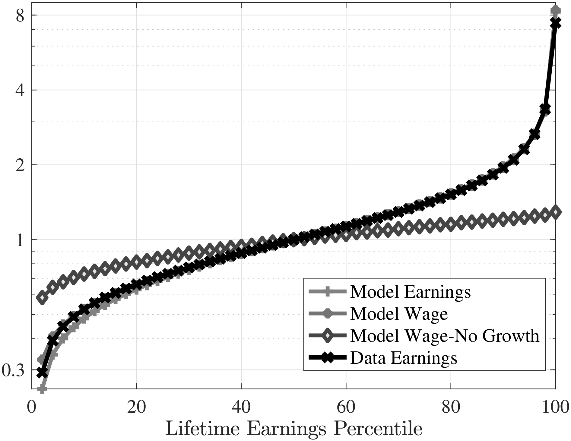
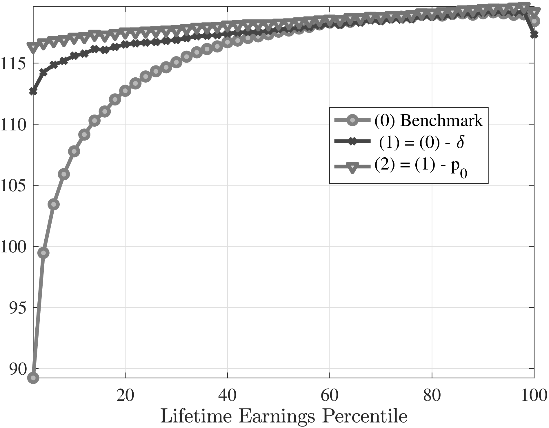
Notes: “Model Wage–No Growth” corresponds to an experiment that shuts down the heterogeneity in \(\beta\), eliminates search frictions (\(\delta =0,\lambda _{0}=1,\lambda _{1}=0\)), removes idiosyncratic shocks and makes the firm distribution degenerate. In this specification, the only source of wage (and earnings) differences is permanent ability, \(\alpha\). Each series is normalized so that it takes a value of 1 for the median group.
6.2 Decomposing Lifecycle Wage Growth Differences
Recall that in the model wage growth can differ across individuals due to differences in the ability to accumulate human capital, ex-ante and ex-post differences in unemployment risk, and the quality and quantity of offers on and off the job. To assess the relative roles of these factors in lifetime wage growth differences, we shut down each component one after another, until we eliminate all differences, again keeping the composition of the LE groups the same with our benchmark (Figure 10a).34
We start by eliminating the differences in unemployment risk, which we accomplish by shutting off differences in job loss and job finding rates together (\(\delta ^{a}(\alpha _{i})=\delta ^{a}(0\)) and \(\lambda _{0}^{a}(\alpha _{i})=\lambda _{0}^{a}(0)\)). Heterogeneity in unemployment risk has a marked effect on wage growth differences between the bottom and median LE workers, and to a lesser degree above the median (series (1) in Figure 10a). Specifically, slightly more than 50% of wage growth differences at the bottom would diminish, if the workers at the bottom had job loss and job finding rates similar to those of the median LE workers.35
High unemployment rates of low-income individuals (Figure 9b) not only prevent them from accumulating human capital but also lead to depreciation in human capital during unemployment. Furthermore, a higher incidence of unemployment prevents bottom LE workers from climbing the job ladder. Figure 10b shows the contributions of human capital, search capital and negotiation rents to the wage growth differences between the bottom and median LE workers.36 Differences in human capital accumulation account for almost 70% of the wage growth differences between these two groups. And, lower human capital accumulation at the bottom of the LE distribution is not because these workers have much lower returns to experience but because they accumulate less experience due to their higher prevalence of unemployment spells. The remaining difference in wage growth between bottom and median LE workers is essentially due to the accumulation of search capital (i.e., working for more productive firms). The contribution of the negotiation capital is very small and negative, meaning that workers at the bottom experience larger growth in their piece rate compared to those at the median. This is because higher LE workers are employed at more productive firms, which are hard to poach from, and, in turn, increases in wages due to outside offers are smaller for them.37 Eliminating unemployment risk brings down the differences in human and search capital accumulation, and thus differences in wage growth, by around 65%.
Job loss and job finding differences matter much less at the upper half of the distribution, because these workers have fairly low unemployment risk to begin with. The only exception is the top earners, who have a slightly higher job loss risk, thus, eliminating this difference would actually raise their income growth further by around 20 log points.
Recall that LE groups also display sizable differences in their contact rates \(\lambda _{1}\). In contrast to the job loss and job finding rates, these differences have a smaller effect on lifetime wage growth differences (Figure 10a). Specifically, eliminating differences in contact rates would close an additional 20% of the wage growth gap between the bottom and the median, with essentially no effect at the top. All of this effect is due to the closing of search capital differences. Namely, endowing bottom LE individuals with the contact rate of median LE individuals allows bottom LE workers to climb to better jobs. These two experiments show that eliminating differences in job ladder risk can go a long way in ameliorating the labor market experiences of bottom LE workers and eliminate more than 70% of the differences in wage growth with median LE workers.
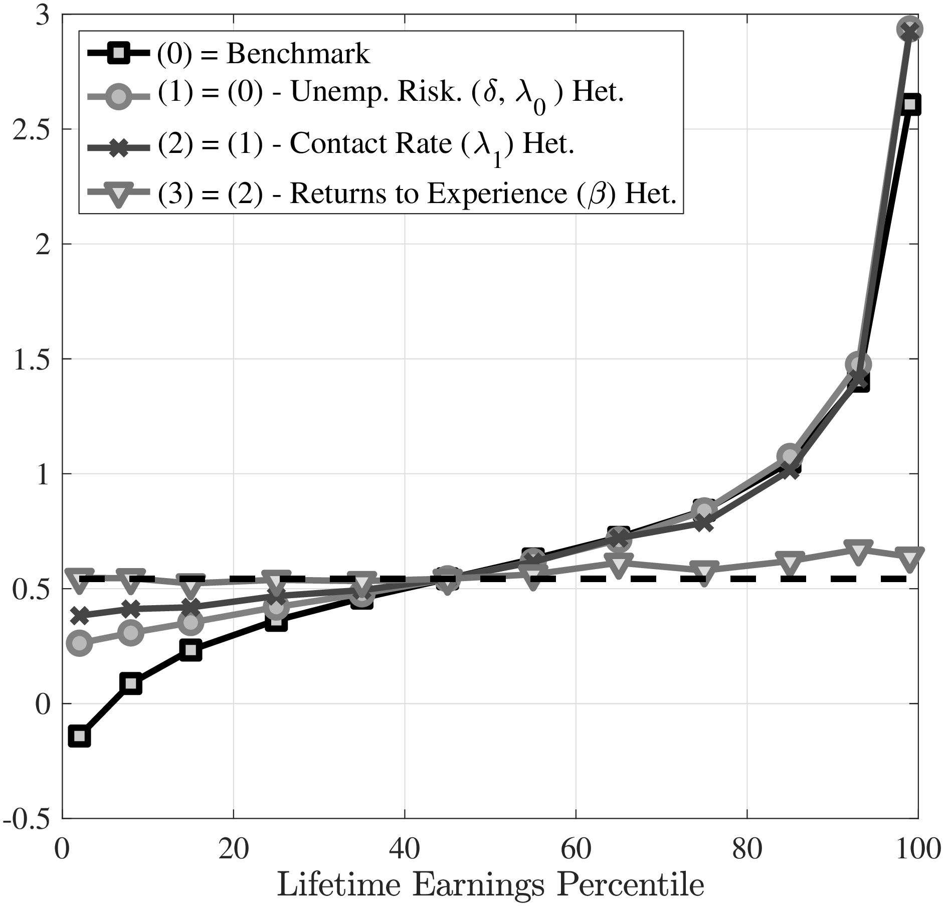
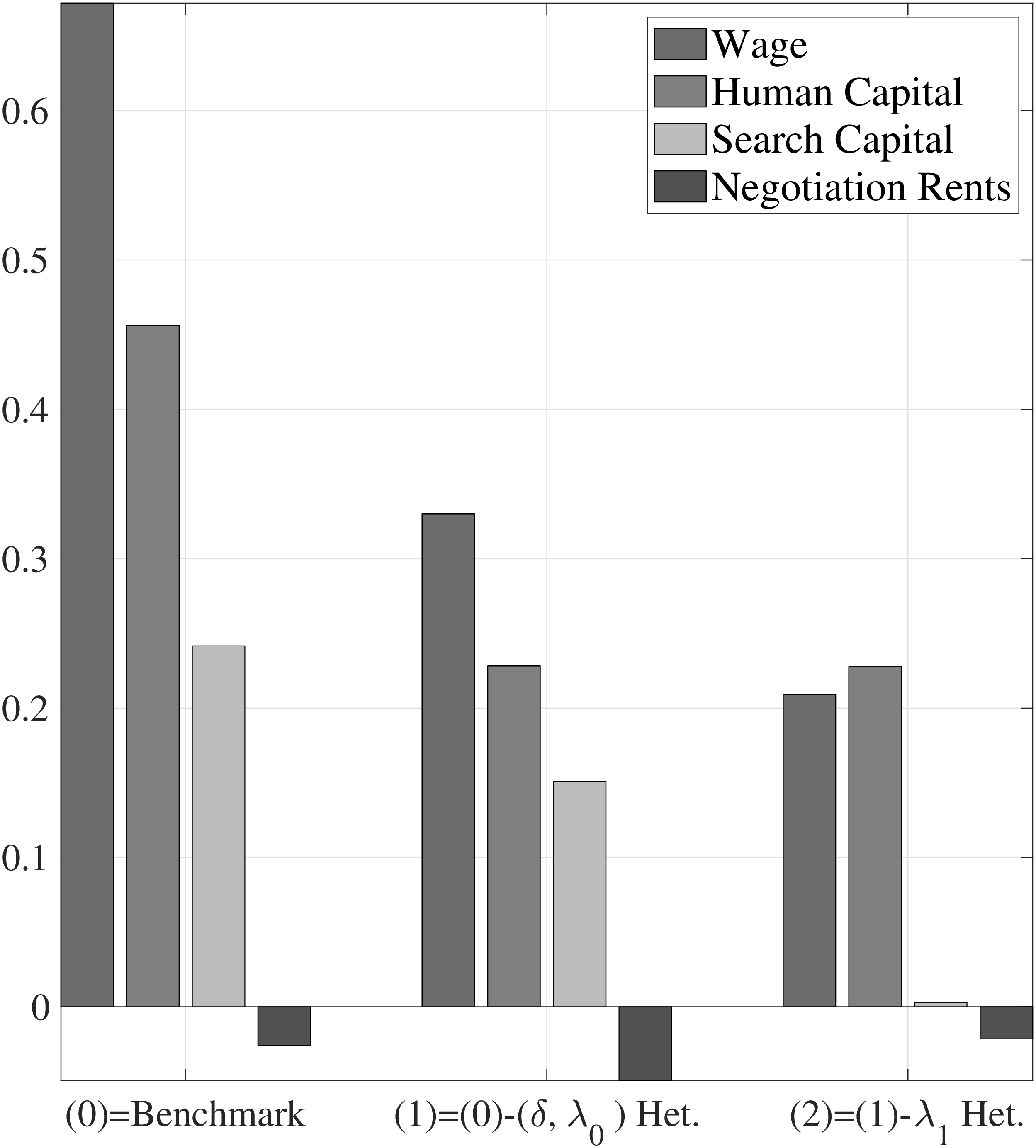
Notes: The left panel decomposes the differences in lifetime wage growth: The black line shows the benchmark wage growth; the circled red, the blue, and the green lines cumulatively eliminate ex-ante heterogeneity in job loss and job finding rates, in contact rate, and in returns to experience, respectively. Black dashed line shows the lifetime wage growth after eliminating all ex-ante heterogeneity and shutting down shocks. The right panel decomposes the average lifetime log wage growth differences between bottom and median LE workers into human capital, search capital and negotiation rents.
Next, we turn to the role of heterogeneity in returns to experience. To this end, we assign all workers’ \(\beta\) to the average, after which we are left with only idiosyncratic productivity shocks and the random realizations of labor market shocks (Figure 10a). Recall that \(\beta\) is relatively flatter in the bottom two-thirds and increases steeply towards the top of the LE distribution (Figure 5a). Thus, eliminating differences in returns to experience has an effect across the entire LE distribution but the largest effect is by far on the top LE earners. Together with the fact that job ladder risk plays a smaller role for top earners, the reason why top earners experience a much larger wage growth than the median is primarily because they have much higher returns to experience thereby accumulating human capital at a higher pace. In the bottom half of the LE distribution, \(\beta\) heterogeneity can explain only around 25% of wage growth differences and the primary source of heterogeneity is in job ladder risk.
Intuition behind the quantitative results. Which feature of the data tells the model that human capital accumulation is more important at the upper half of the LE distribution and vice versa at the bottom half? While all targeted moments are informative, we argue that the differences between income growth of job stayers and switchers are key. To see this, note that human capital is capitalized into wages in all firms. Therefore, wage growth always reflects a worker’s human capital accumulation, regardless of whether he stays with the current employer or switches to a new one. If the data show a high wage growth for a group of workers relative to median workers regardless of job switching, as is the case in the data for higher LE individuals (Figure 2c), the model infers a high returns to experience.
The difference in earnings growth between stayers and switchers is informative about the role of job ladder risk. If a group of workers experience lower growth when switching than they do when they stay with the same employer, the model rationalizes this by inferring a poor job ladder, due to a high job loss or a low job finding rate. At the bottom of the LE distribution, job switchers experience much smaller earnings growth compared to stayers, consistent with our finding that the job ladder component is more important for explaining their lackluster lifetime growth relative to the median.
Initial conditions versus shocks. Our findings also shed new light on the relative roles of ex-ante heterogeneity in initial conditions and ex-post shocks (Keane and Wolpin (1997); Huggett et al. (2011)). Figure 10a shows a negligible role for luck—idiosyncratic productivity and job ladder shocks—in lifetime wage growth differences after removing all ex-ante heterogeneity. On average, above median LE workers are somewhat more lucky, but this has a very small quantitative effect. However, Figure 10a shows differences between LE groups and average out possible within group differences from ex-post shocks.
For a more precise measure, we decompose the variance of log lifetime earnings into “ex-ante heterogeneity” and “ex-post shocks” components. 81% of the variation in lifetime earnings is due to ex-ante heterogeneity in initial conditions, substantially higher than the 61% that Huggett et al. (2011) find from a similar exercise. Their Ben-Porath model does not feature job ladder dynamics and attributes income changes due to job ladder shocks (e.g., job loss, etc.) to productivity shocks. Through the lens of their model, bottom LE workers are just unlucky and often draw negative productivity shocks. In our model they have high ex-ante unemployment risk. Thus, the higher role for initial conditions in our model stems from richer worker heterogeneity, which more precisely captures the source of inequality in the bottom half.
7 Conclusion
We investigated the determinants of lifetime earnings inequality by focusing on heterogeneity in job ladder dynamics and on-the-job learning. Empirically, we showed that i) lower LE workers switch jobs more often, mainly driven by higher nonemployment, ii) earnings growth for job stayers is similar in the bottom two thirds of the LE distribution, iii) while rising strongly with LE for job switchers. Estimating a model featuring rich worker and firm heterogeneity, we found large differences in ex-ante job ladder risk across workers. These differences account for 75% of the lifetime wage growth differential below the median of the LE distribution. Above the median, almost all lifetime wage growth differences are a result of Pareto-distributed learning ability.
We conclude that different economic forces are driving the inequality in different parts of the LE distribution. These differences have important implications for the design of insurance policies. For example, Golosov et al. (2013) show that optimal redistribution looks very different when differences in labor income emanate from search frictions as opposed to differences in workers’ productivity. Similarly, the effects of the monetary policy can be heterogenous as it may affect workers job ladder risk differently across the income distribution, thereby leading to differences in wage growth.
An emerging literature studies the effects of firms’ power in setting wages. Firms can hire and retain workers at wages lower than the competitive fringe if they are large in a market (Berger et al. (2019); Jarosch et al. (2019)) or if they do not face much competition from other employers, either due to contractual restrictions on job mobility (Johnson et al. (2019)) or other frictions. One interpretation of the estimated differences in outside contacts is about employers’ ability to restrict poaching. Through this lens, our results suggest that firms are better able to restrict poaching for low-skill workers and have more power over them. This interpretation is consistent with Caldwell and Danieli (2018), who find much less competitive pressure for low-skill workers.
Lastly, our analysis has focused on worker differences. However, some of the differences could be a characteristic of jobs rather than workers. Jarosch (2015) focuses on firm heterogeneity in job stability. More broadly, firms might contribute to wage growth heterogeneity by providing different learning environments (e.g., Herkenhoff et al. (2018); Gregory (2019)). To fully understand the role of firms and workers in wage dynamics, a unified approach is necessary, which we leave for future work (e.g., Koffi et al. (2022)).
References
Abrahám, A., Alvarez-Parra, F. and Forstner, S. (2016). The effects of moral hazard on wage inequality in a frictional labor market. Unpublished working paper.
Ahn, H. J. and Hamilton, J. D. (2020). Heterogeneity and unemployment dynamics. Journal of Business & Economic Statistics, 38 (3), 554–569.
—, Hobijn, B. and Şahin, A. (2022). The dual us labor market uncovered.
Altonji, J. G. and Segal, L. M. (1996). Small-sample bias in GMM estimation of covariance structures. Journal of Business & Economic Statistics, 14 (3), 353–366.
Andrews, I., Gentzkow, M. and Shapiro, J. M. (2017). Measuring the Sensitivity of Parameter Estimates to Estimation Moments*. The Quarterly Journal of Economics, 132 (4), 1553–1592.
Atkinson, A. B., Piketty, T. and Saez, E. (2011). Top incomes in the long run of history. Journal of Economic Literature, 49 (1), 3–71.
Bagger, J., Fontaine, F., Postel-Vinay, F. and Robin, J.-M. (2014). Tenure, experience, human capital and wages: A tractable equilibrium search model of wage dynamics. American Economic Review, 104 (6), 1551–1596.
— and Lentz, R. (2014). An empirical model of wage dispersion with sorting. The Review of Economic Studies.
Barlevy, G. (2008). Identification of search models using record statistics. The Review of Economic Studies, 75 (1), 29–64.
Ben-Porath, Y. (1967). The production of human capital and the life cycle of earnings. Journal of Political Economy, 75 (4), 352–365.
Berger, D. W., Herkenhoff, K. F. and Mongey, S. (2019). Labor Market Power. Tech. rep., National Bureau of Economic Research.
Blanchard, O. J. (1985). Debt, deficits, and finite horizons. Journal of Political Economy, 93 (2), 223–247.
Bonhomme, S., Lamadon, T. and Manresa, E. (2017). A distributional framework for matched employer employee data. Unpublished manuscript, University of Chicago.
Bowlus, A. J. and Liu, H. (2013). The contributions of search and human capital to earnings growth over the life cycle. European Economic Review, 64, 305–331.
Burdett, K. and Mortensen, D. T. (1998). Wage differentials, employer size, and unemployment. International Economic Review, 39 (2), 257–73.
Cahuc, P., Postel-Vinay, F. and Robin, J.-M. (2006). Wage bargaining with on-the-job search: Theory and evidence. Econometrica, 74 (2), 323–364.
Cairo, I. and Cajner, T. (2017). Human capital and unemployment dynamics: Why more educated workers enjoy greater employment stability. The Economic Journal, 128 (609), 652–682.
Caldwell, S. and Danieli, O. (2018). Outside options in the labor market. Unpublished manuscript.
Caucutt, E. M. and Lochner, L. (2020). Early and late human capital investments, borrowing constraints, and the family. Journal of Political Economy, 128 (3), 1065–1147.
Chetty, R. (2008). Moral hazard versus liquidity and optimal unemployment insurance. Journal of political Economy, 116 (2), 173–234.
Deaton, A. and Paxson, C. (1994). Intertemporal choice and inequality. Journal of Political Economy, 102 (3), 437–67.
Faberman, R. J., Mueller, A. I., Şahin, A. and Topa, G. (2017). Job search behavior among the employed and non-employed. Tech. rep., National Bureau of Economic Research.
Fujita, S. and Moscarini, G. (2017). Recall and unemployment. American Economic Review, 107 (12), 3875–3916.
Gabaix, X., Lasry, J.-M., Lions, P.-L. and Moll, B. (2016). The dynamics of inequality. Econometrica, 84 (6), 2071–2111.
Gathmann, C. and Schönberg, U. (2010). How general is human capital? a task-based approach. Journal of Labor Economics, 28 (1), 1–49.
Golosov, M., Maziero, P. and Menzio, G. (2013). Taxation and redistribution of residual income inequality. Journal of Political Economy, 121 (6), 1160–1204.
Gregory, V. (2019). Firms as learning environments: Implications for earnings dynamics and job search. Unpublished Manuscript.
—, Menzio, G. and Wiczer, D. G. (2021). The Alpha Beta Gamma of the Labor Market. Tech. rep., National Bureau of Economic Research.
Guvenen, F., Kaplan, G. and Song, J. (2014a). The glass ceiling and the paper floor: Gender differences among top earners, 1981-2012. Tech. rep., National Bureau of Economic Research.
—, —, — and Weidner, J. (2017). Lifetime incomes in the United States over six decades. Tech. rep., National Bureau of Economic Research.
—, Karahan, F., Ozkan, S. and Song, J. (2021). What do data on millions of us workers reveal about lifecycle earnings dynamics? Econometrica, 89 (5), 2303–2339.
— and Ozkan, S. (2021). TikTak: A multistart global optimization algorithm, https://github.com/serdarozkan/TikTak.
—, — and Song, J. (2014b). The nature of countercyclical income risk. Journal of Political Economy, 122 (3), 621–660.
Hall, R. E. and Kudlyak, M. (2022). Churn and Stability: The Remarkable Heterogeneity of Flows among Employment, Job Search, and Non-Market Activities in the US Population. Tech. rep.
Haltiwanger, J., Hyatt, H. R., McEntarfer, E., Sousa, L. and Tibbets, S. (2014). Firm age and size in the longitudinal employer-household dynamics data. US Census Bureau Center for Economic Studies Paper No. CES-WP-14-16.
Halvorsen, E., Holter, H., Ozkan, S. and Storesltetten, K. (2019). Dissecting Idiosyncratic Income Risk: Evidence from Norwegian Registry Data,. Tech. rep., Technical report, mimeo.
Heckman, J. J. (1976). A life-cycle model of earnings, learning, and consumption. Journal of political economy, 84 (4, Part 2), S9–S44.
Herkenhoff, K., Lise, J., Menzio, G. and Phillips, G. M. (2018). Production and Learning in Teams. Tech. rep., National Bureau of Economic Research.
Hubmer, J. (2018). The job ladder and its implications for earnings risk. Review of Economic Dynamics, 29, 172–194.
Huggett, M. and Kaplan, G. (2016). How large is the stock component of human capital? Review of Economic Dynamics, 22, 21–51.
—, Ventura, G. and Yaron, A. (2011). Sources of lifetime inequality. American Economic Review, 101 (7), 2923–54.
Jarosch, G. (2015). Searching for Job Security and the Consequences of Job Loss. Working paper, Princeton University.
—, Nimczik, J. S. and Sorkin, I. (2019). Granular Search, Market Structure, and Wages. Tech. rep., National Bureau of Economic Research.
— and Pilossoph, L. (2018). Statistical Discrimination and Duration Dependence in the Job Finding Rate. The Review of Economic Studies.
Johnson, M. S., Lavetti, K. and Lipsitz, M. (2019). The labor market effects of legal restrictions on worker mobility. Available at SSRN 3455381.
Jolivet, G., Postel-Vinay, F. and Robin, J.-M. (2006). The empirical content of the job search model: Labor mobility and wage distributions in Europe and the U.S. In Structural Models of Wage and Employment Dynamics, Emerald Group Publishing Limited, pp. 269–308.
Jones, C. I. and Kim, J. (2018). A Schumpeterian model of top income inequality. Journal of Political Economy, 126 (5), 1785–1826.
Jovanovic, B. (1979). Job matching and the theory of turnover. Journal of Political Economy, 87 (5), 972–90.
Jung, P. and Kuhn, M. (2018). Earnings Losses and Labor Mobility Over the Life Cycle. Journal of the European Economic Association, 17 (3), 678–724.
Kaplan, G. (2012). Inequality and the life cycle. Quantitative Economics, 3 (3), 471–525.
Keane, M. P. and Wolpin, K. I. (1997). The career decisions of young men. Journal of political Economy, 105 (3), 473–522.
Koffi, M., Ozkan, S., Salgado, S. and Weissler, M. (2022). High risk workers and high risk firms. Working Paper.
Krolikowski, P. (2017). Job ladders and earnings of displaced workers. American Economic Journal: Macroeconomics, 9 (2), 1–31.
Lazear, E. P. and Rosen, S. (1981). Rank-order tournaments as optimum labor contracts. Journal of Political Economy, 89 (5), 841–864.
Lentz, R., Piyapromdee, S., Robin, J.-M. et al. (2018). On worker and firm heterogeneity in wages and employment mobility: Evidence from anish register data. PIER Discussion Papers, 91.
Lise, J. (2013). On the job search and precautionary savings. Review of Economic Studies, 80, 1086–1113.
—, Meghir, C. and Robin, J.-M. (2016). Matching, sorting and wages. Review of Economic Dynamics, 19, 63–87.
Mincer, J. (1974). Schooling, Experience and Earnings. New York: Columbia University Press.
Morchio, I. (2020). Work histories and lifetime unemployment. International Economic Review, 61 (1), 321–350.
Neal, D. and Rosen, S. (2000). Theories of the distribution of earnings. Handbook of Income Distribution, 1, 379–427.
Olsen, A. and Hudson, R. (2009). Social Security Administration’s master earnings file: Background information. Social Security Bulletin, 69 (3), 29–46.
Panis, C., Euller, R., Grant, C., Bradley, M., Peterson, C. E., Hirscher, R. and Stinberg, P. (2000). SSA Program Data User’s Manual. Baltimore, MD: Social Security Administration.
Pastorino, E. (2019). Careers in firms: the role of learning and human capital. Tech. rep., mimeo.
Piketty, T. and Saez, E. (2003). Income inequality in the United States: 1913-1998. Quarterly Journal of Economics, 118 (1), 1–39.
Polachek, S. W., Das, T. and Thamma-Apiroam, R. (2015). Micro-and macroeconomic implications of heterogeneity in the production of human capital. Journal of Political Economy, 123 (6), 1410–1455.
Postel-Vinay, F. and Robin, J.-M. (2002). Equilibrium wage dispersion with worker and employer heterogeneity. Econometrica, 70 (6), 2295–2350.
Rubinstein, A. (1982). Perfect equilibrium in a bargaining model. Econometrica: Journal of the Econometric Society, pp. 97–109.
Schaal, E. (2017). Uncertainty and unemployment. Econometrica, 85 (6), 1675–1721.
Shimer, R. (1998). Why is the U.S. unemployment rate so much lower? NBER Macroeconomics Annual, 13, 11–61.
— (2001). The impact of young workers on the aggregate labor market. The Quarterly Journal of Economics, 116 (3), 969–1007.
Song, J., Price, D. J., Guvenen, F., Bloom, N. and Von Wachter, T. (2018). Firming up inequality. The Quarterly Journal of Economics, 134 (1), 1–50.
Sorkin, I. (2018). Ranking firms using revealed preference. The Quarterly Journal of Economics, 133 (3), 1331–1393.
Tanaka, S., Warren, L. and Wiczer, D. (2019). Earnings growth, job flows and churn. Tech. rep.
Topel, R. H. and Ward, M. P. (1992). Job mobility and the careers of young men. The Quarterly Journal of Economics, 107 (2), 439–79.
Van den Berg, G. J. (1990). Search behaviour, transitions to non-participation and the duration of unemployment. The Economic Journal, 100 (402), 842–865.
Von Wachter, T., Song, J. and Manchester, J. (2009). Long-term earnings losses due to mass layoffs during the 1982 recession: An analysis using us administrative data from 1974 to 2004. Unpublished paper, Columbia University.
Zhang, H., Conn, A. R. and Scheinberg, K. (2010). A derivative-free algorithm for least-squares minimization. SIAM Journal on Optimization, 20 (6), 3555–3576.
Anatomy of Lifetime Earnings Inequality: Heterogeneity in Job Ladder Risk vs. Human Capital Serdar Ozkan38
Supplemental Online Appendix
8 Additional Results from the MEF
8.1 Sample Selection
Our initial sample consists of 1,845,640 individuals (Table A.1). About 18% are self-employed in at least one fourth of their working life. About 490,000 are eliminated, as they do not satisfy the minimum years of employment criterion. We exclude close to 160,000 (27,000) individuals due to consecutive nonemployment(self-employment). This procedure leaves us with a final sample of 840,194 individuals for whom we have at least 31 years of earnings data.
| # individuals dropped | Size after selection | |
| Initial sample | 1,845,640 | |
| # yrs self-employed | 326,822 | 1,518,818 |
| # yrs employed | 489,504 | 1,029,314 |
| consecutive nonemployment | 161,420 | 867,894 |
| consecutive self-employment | 27,700 | 840,194 |
8.2 Moments for Top Earners
| Ratio of lifetime earnings | Relative top income shares | ||||||||
| LE | 25 | 40 | 55 | LE | 25 | 40 | 55 | ||
| \(LE_{50}/LE_{1}\) | 25.5 | 3.3 | 23.8 | 47.8 | S(0.1)/S(1) | 0.29 | 0.24 | 0.31 | 0.38 |
| \(LE_{50}/LE_{5}\) | 14.2 | 2.1 | 12.9 | 25.0 | S(0.2)/S(2) | 0.29 | 0.24 | 0.30 | 0.38 |
| \(LE_{50}/LE_{45}\) | 3.8 | 1.1 | 3.5 | 5.2 | S(1)/S(10) | 0.29 | 0.23 | 0.30 | 0.37 |
| \(LE_{45}/LE_{5}\) | 3.7 | 2.0 | 3.7 | 4.8 | S(2)/S(20) | 0.28 | 0.22 | 0.30 | 0.36 |
| \(LE_{38}/LE_{13}\) | 1.9 | 1.4 | 1.9 | 2.2 | Pareto index, \(\zeta\) | 2.2 | 2.6 | 2.0 | 1.7 |
| \(LE_{5}/LE_{1}\) | 1.8 | 1.6 | 1.8 | 1.9 | |||||
Notes: Left panel: First column shows the ratio of lifetime earnings of selected LE quantiles. The next three
columns show the ratio of average annual earnings at different ages. Right panel shows the ratios of the share of
top incomes for the lifetime earnings distribution and the cross-sectional earnings distribution at various ages.
The bottom row reports the tail index
\(\zeta\)
of each distribution, specified by the following Pareto CDF:
\(P[x>w]~Cw^{-\zeta}.\)
8.2.1 Pareto Tails of the Earnings Distribution
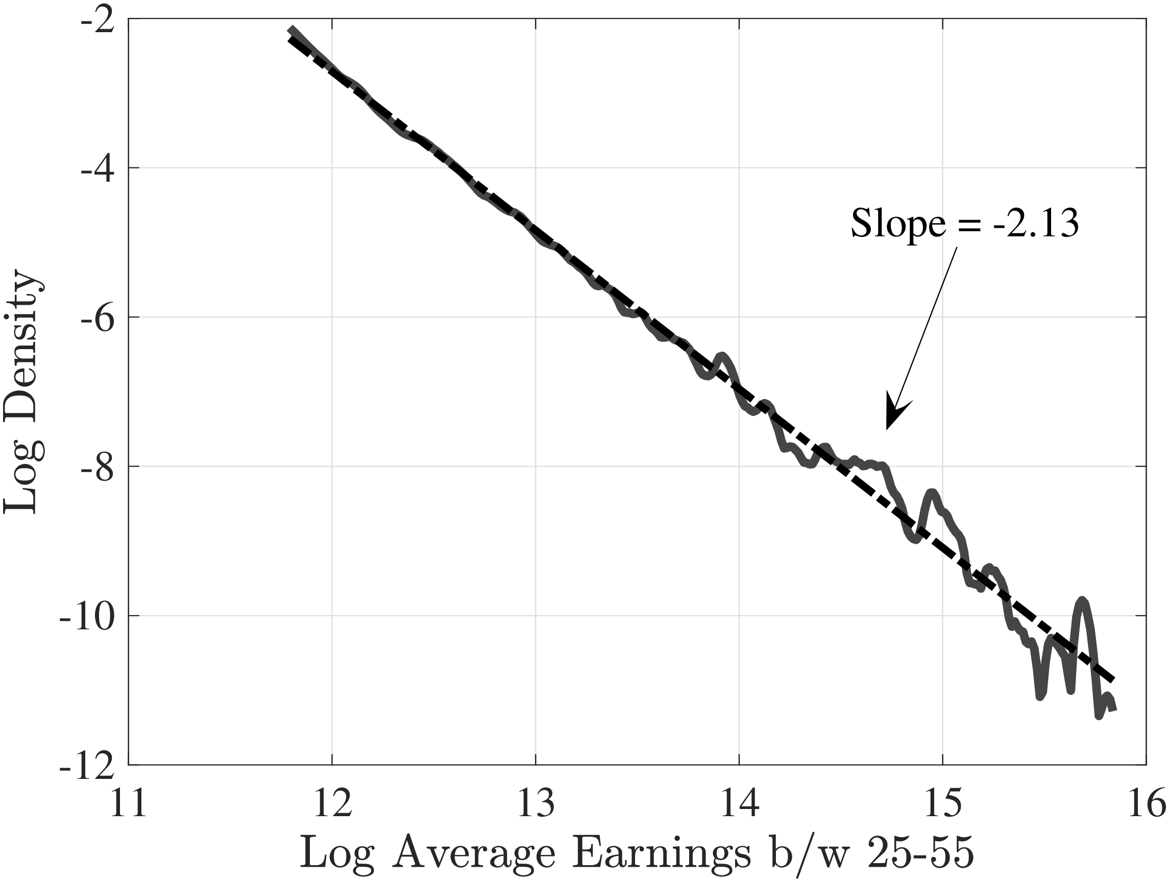
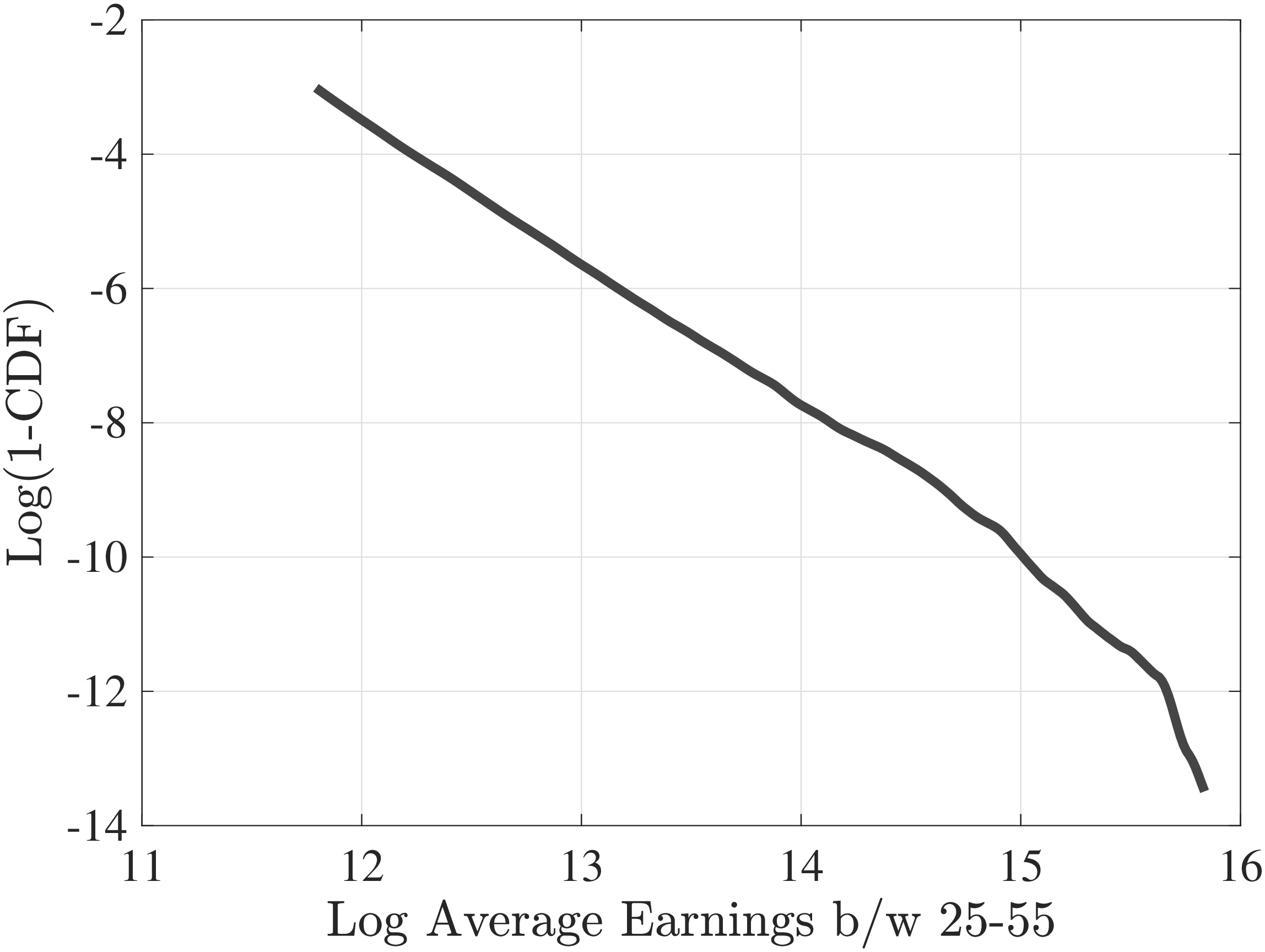
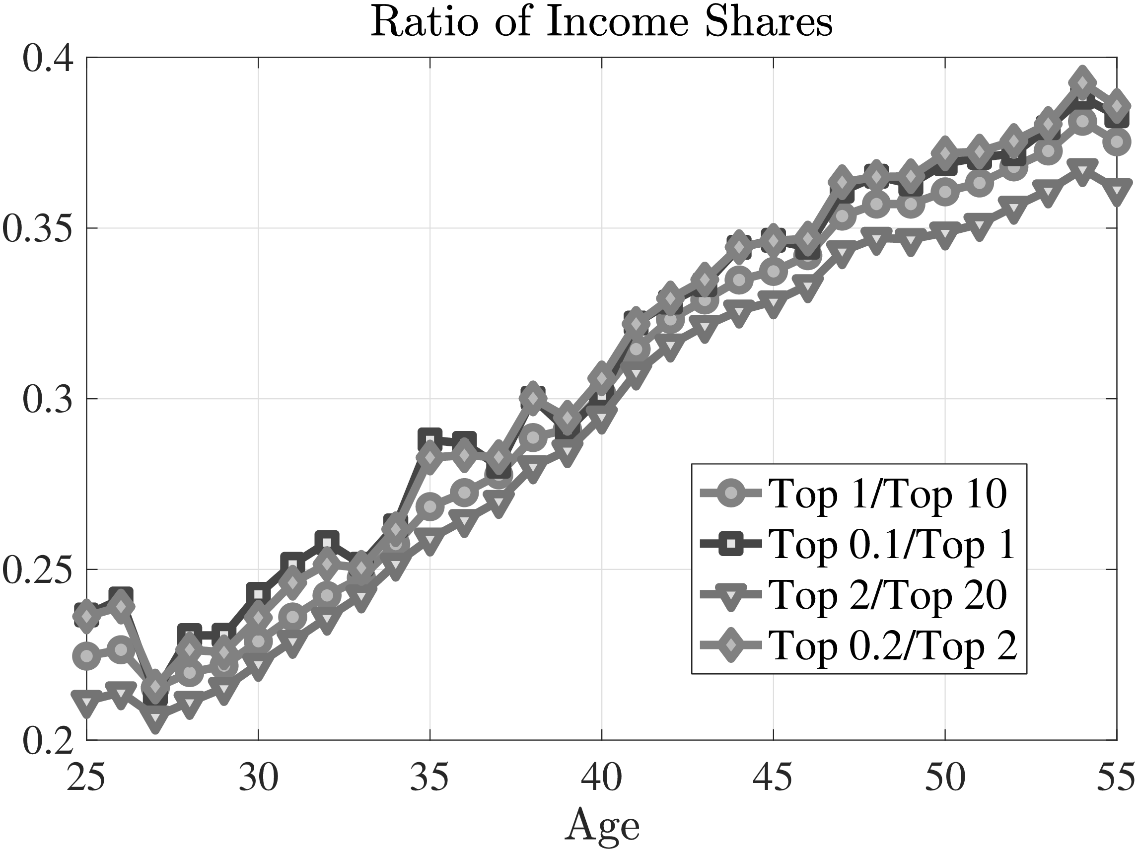
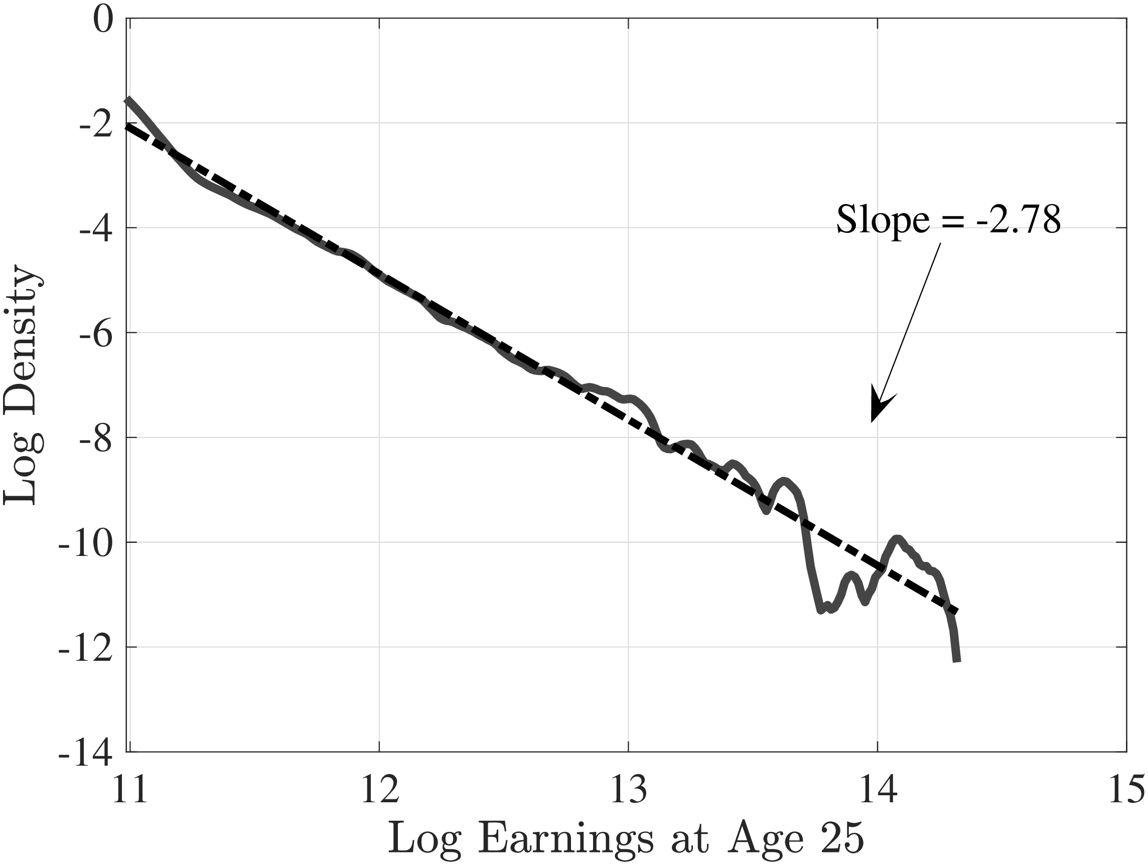
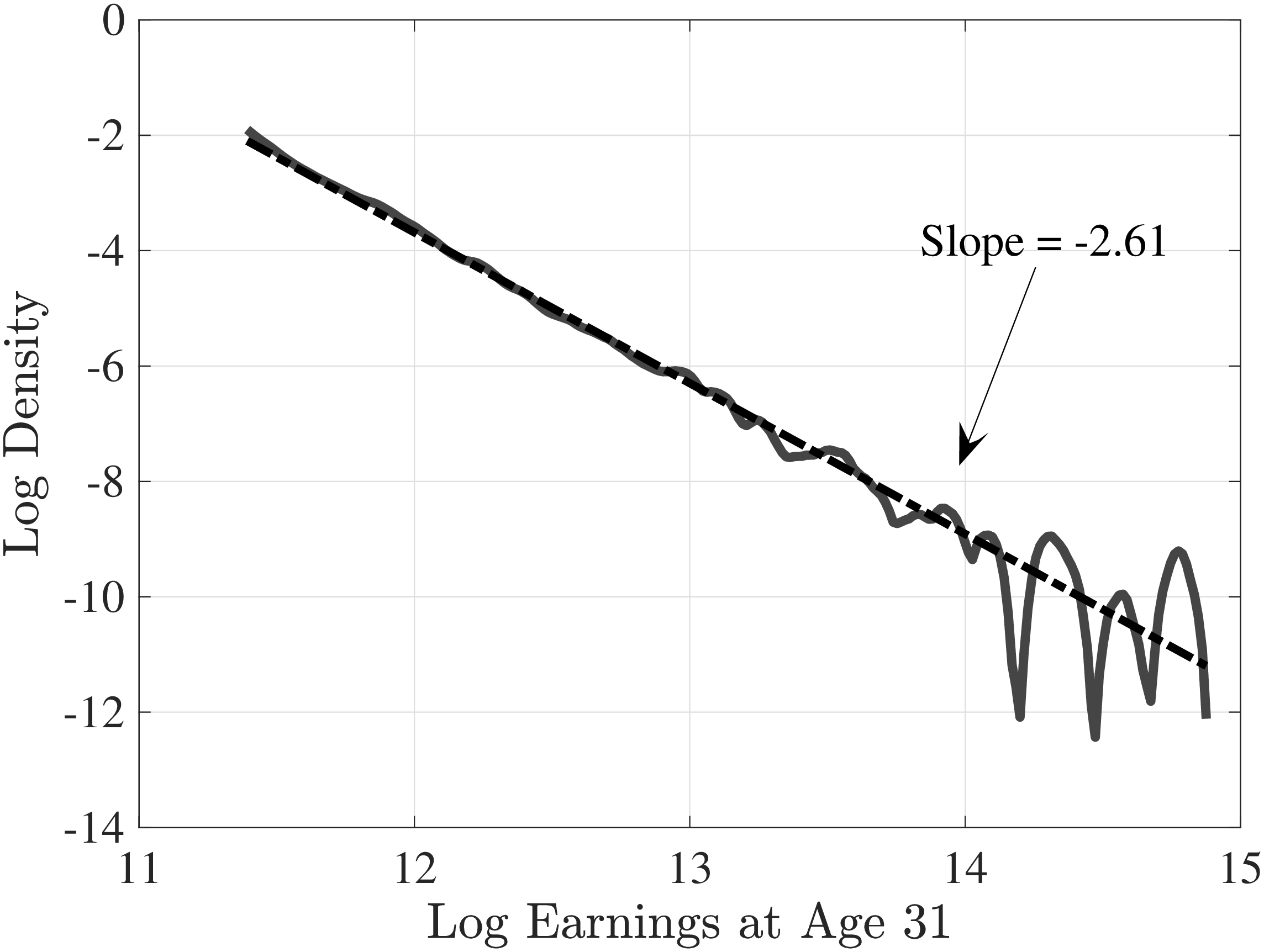
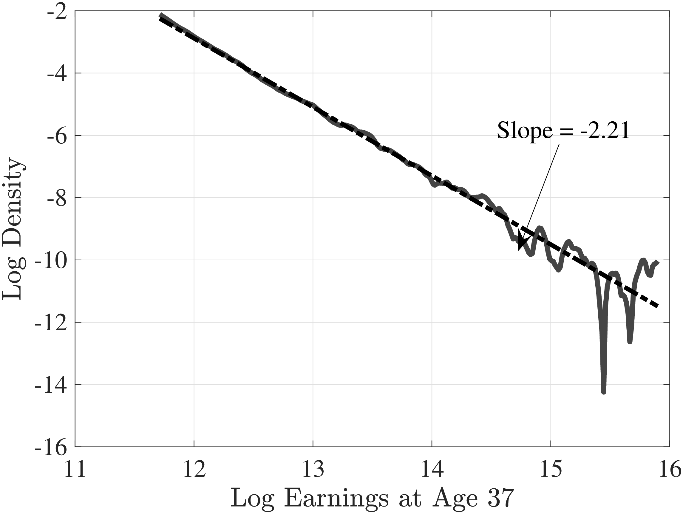
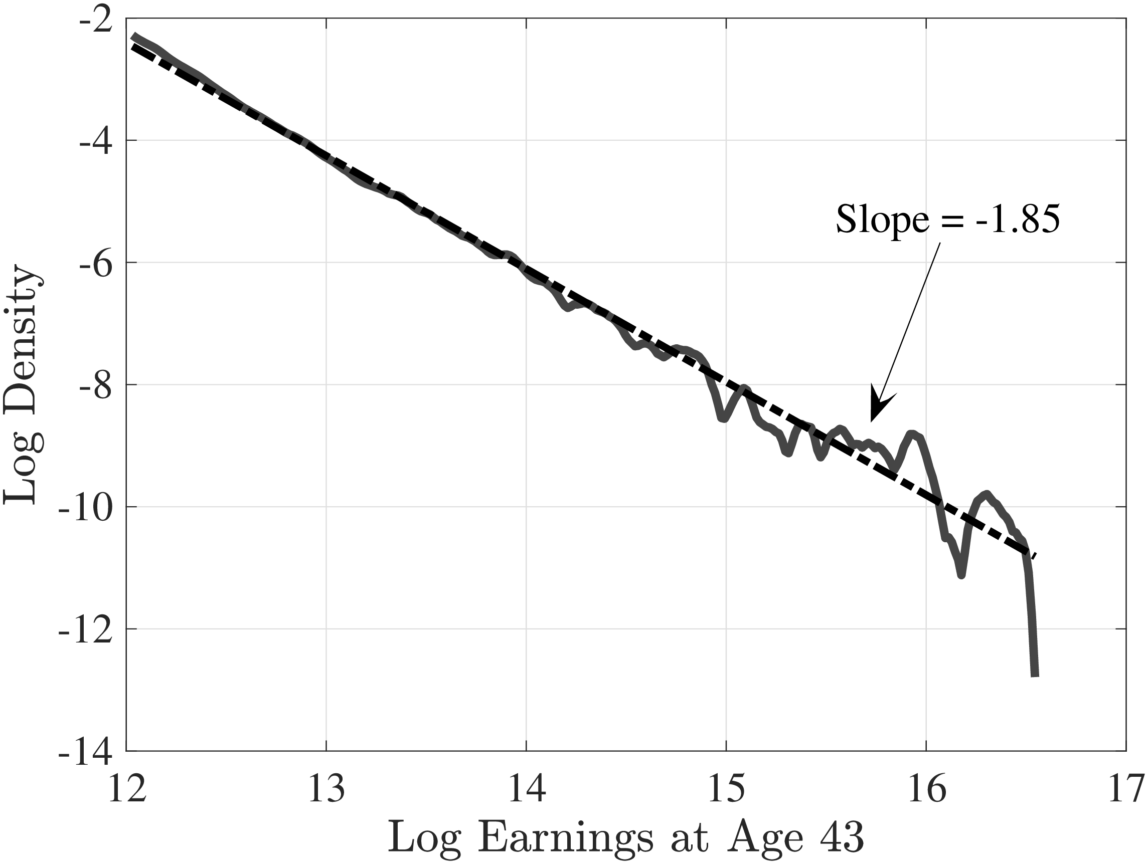
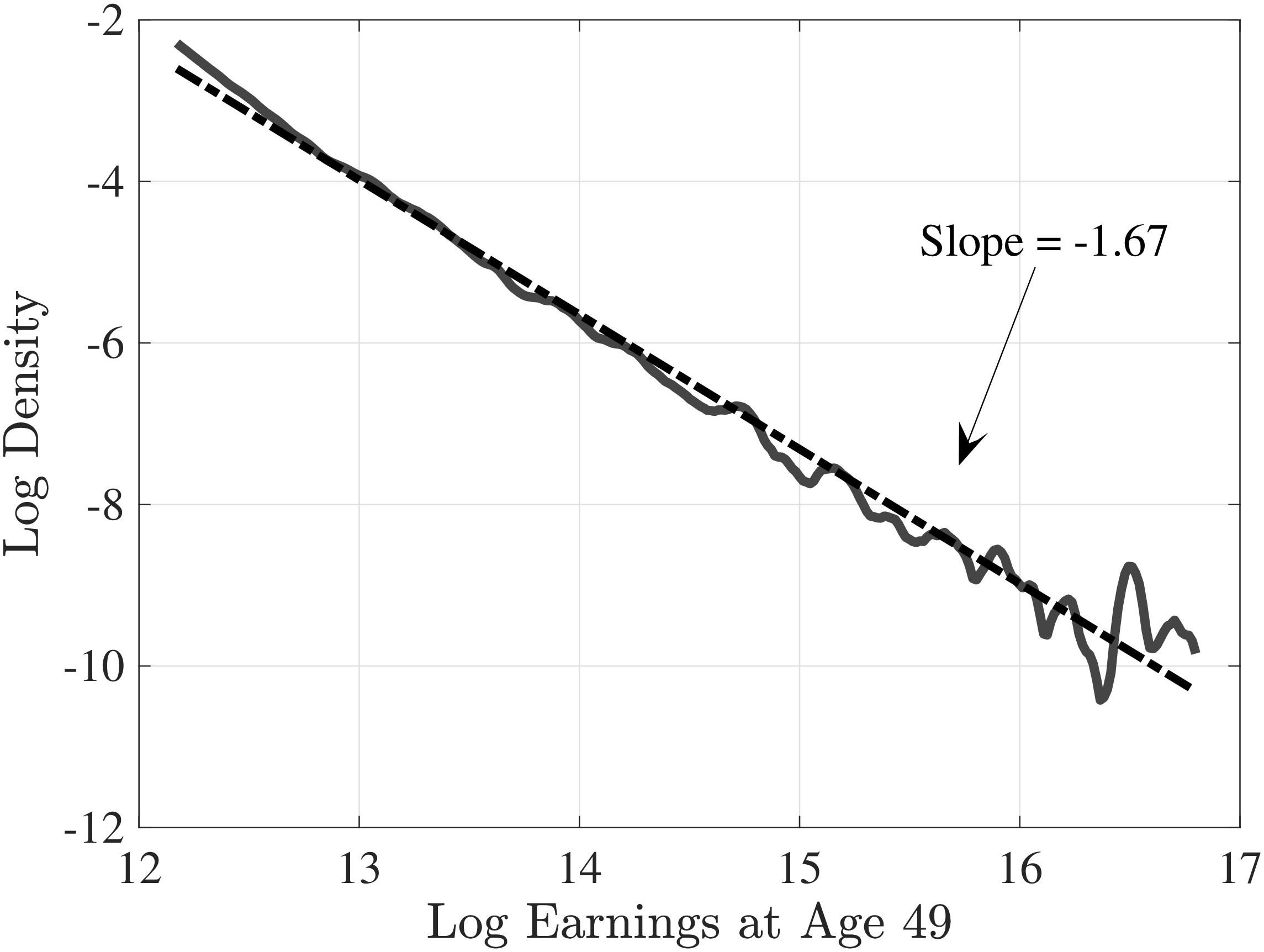
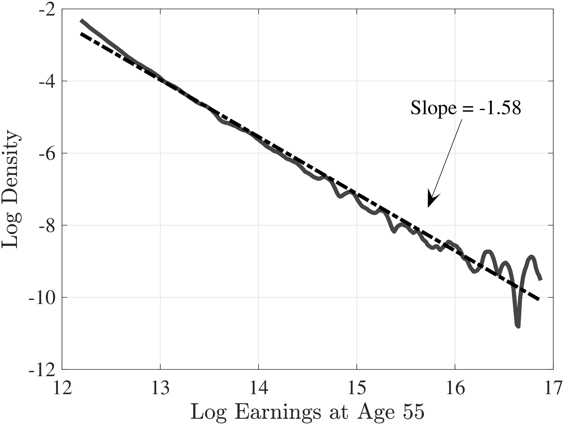
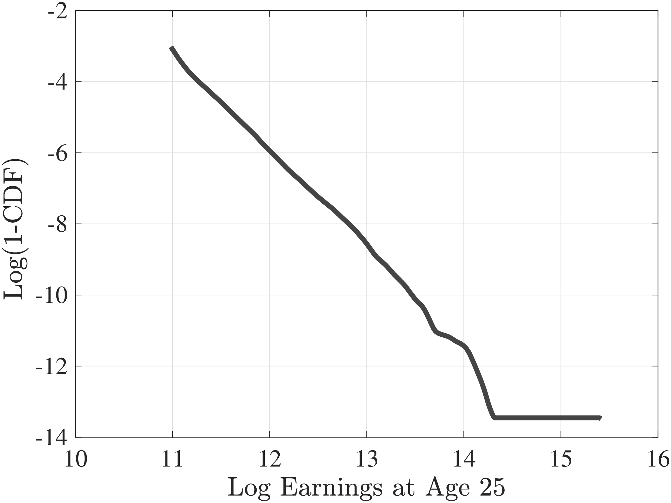
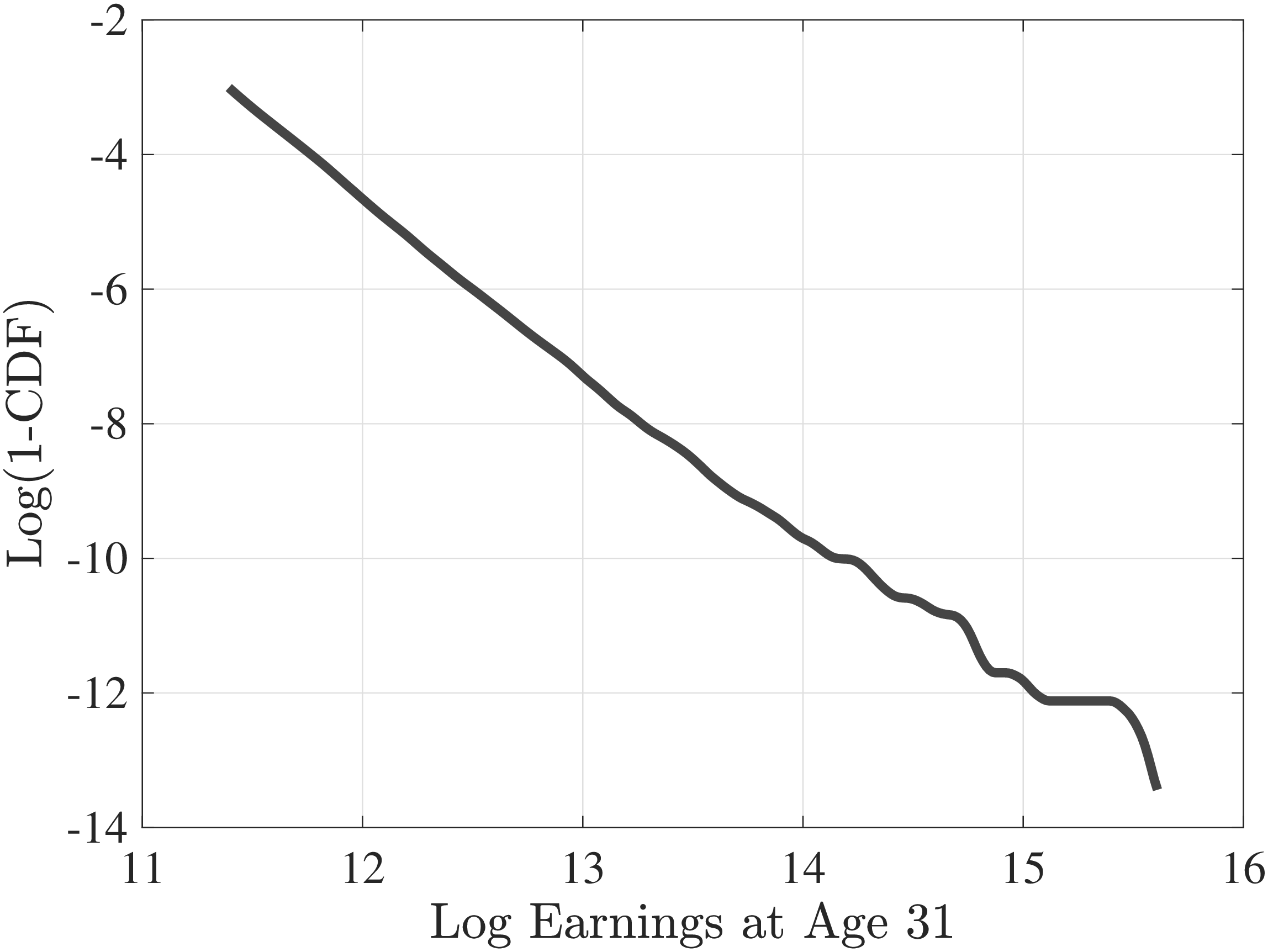
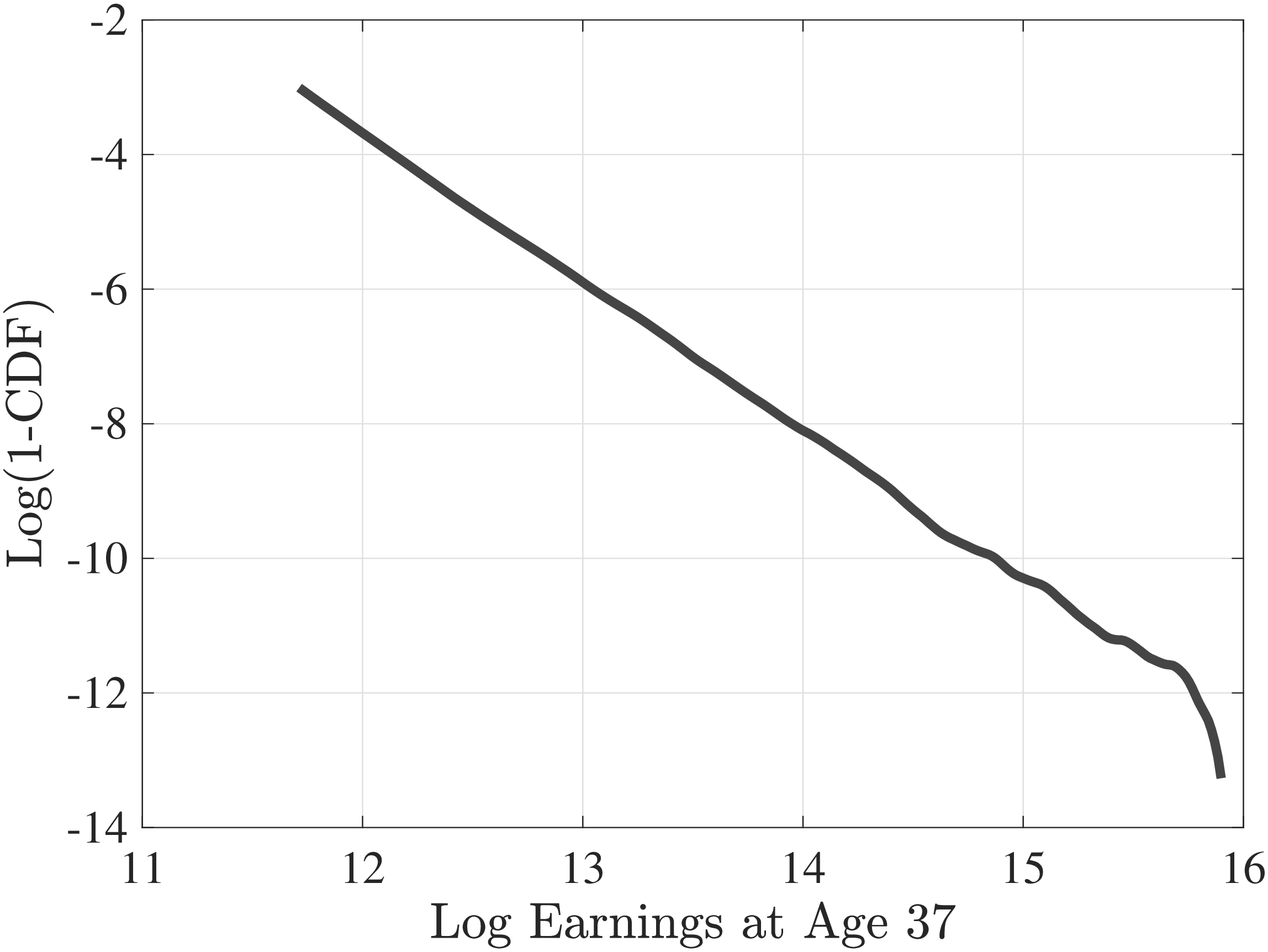
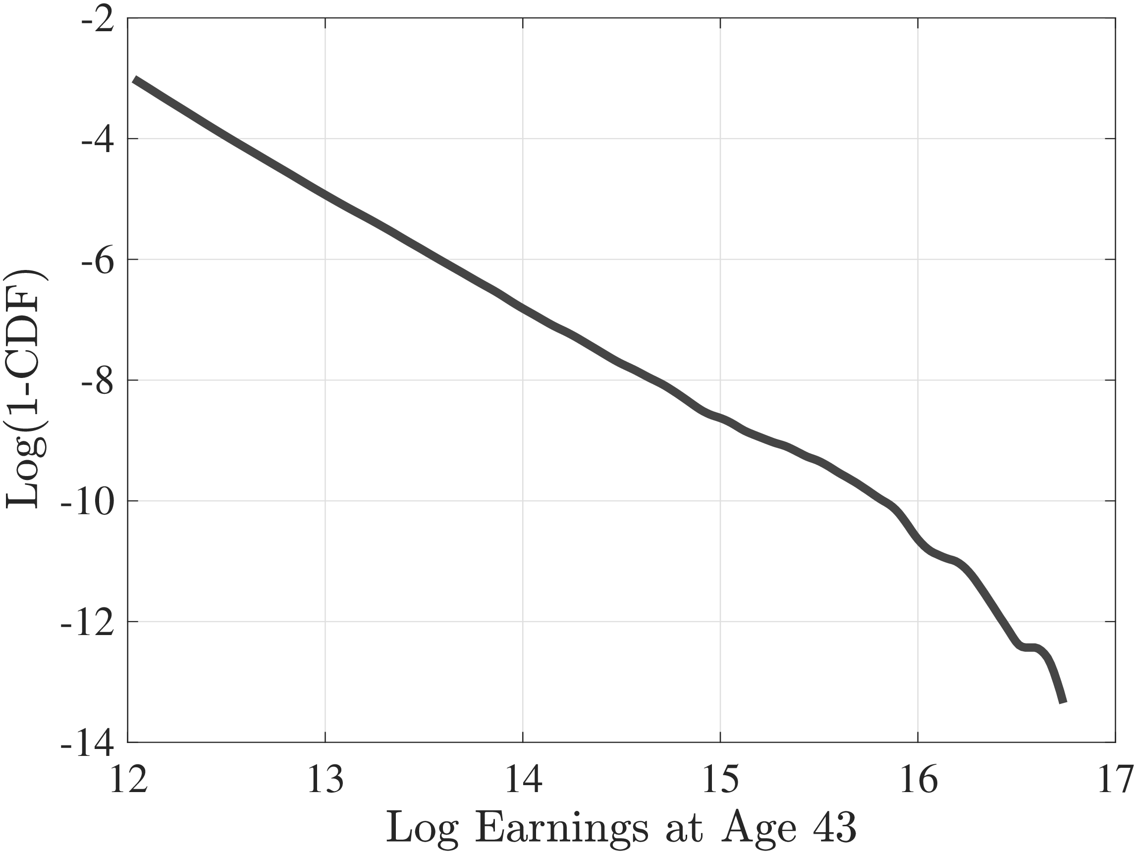
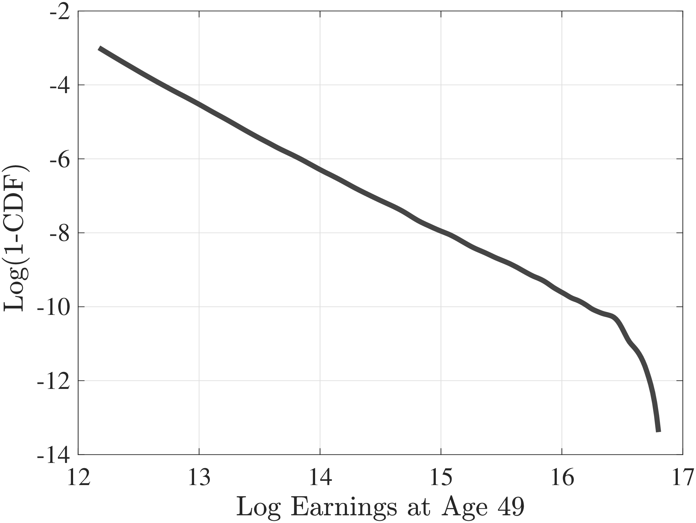
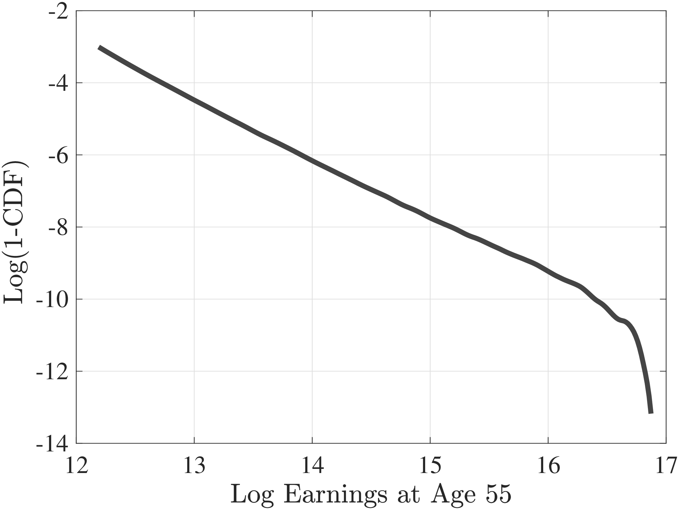
8.2.2 Earnings Growth of Top Earners
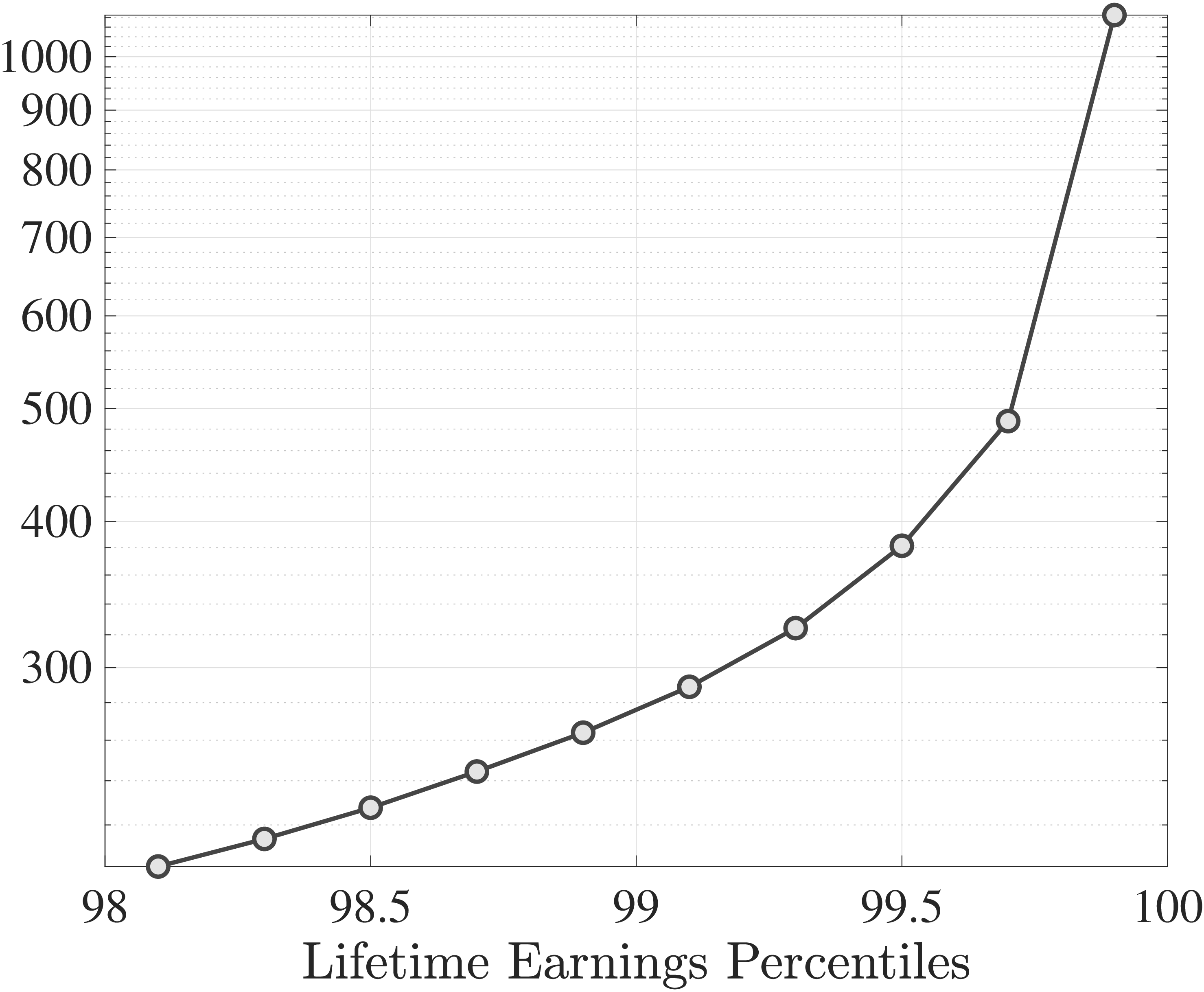
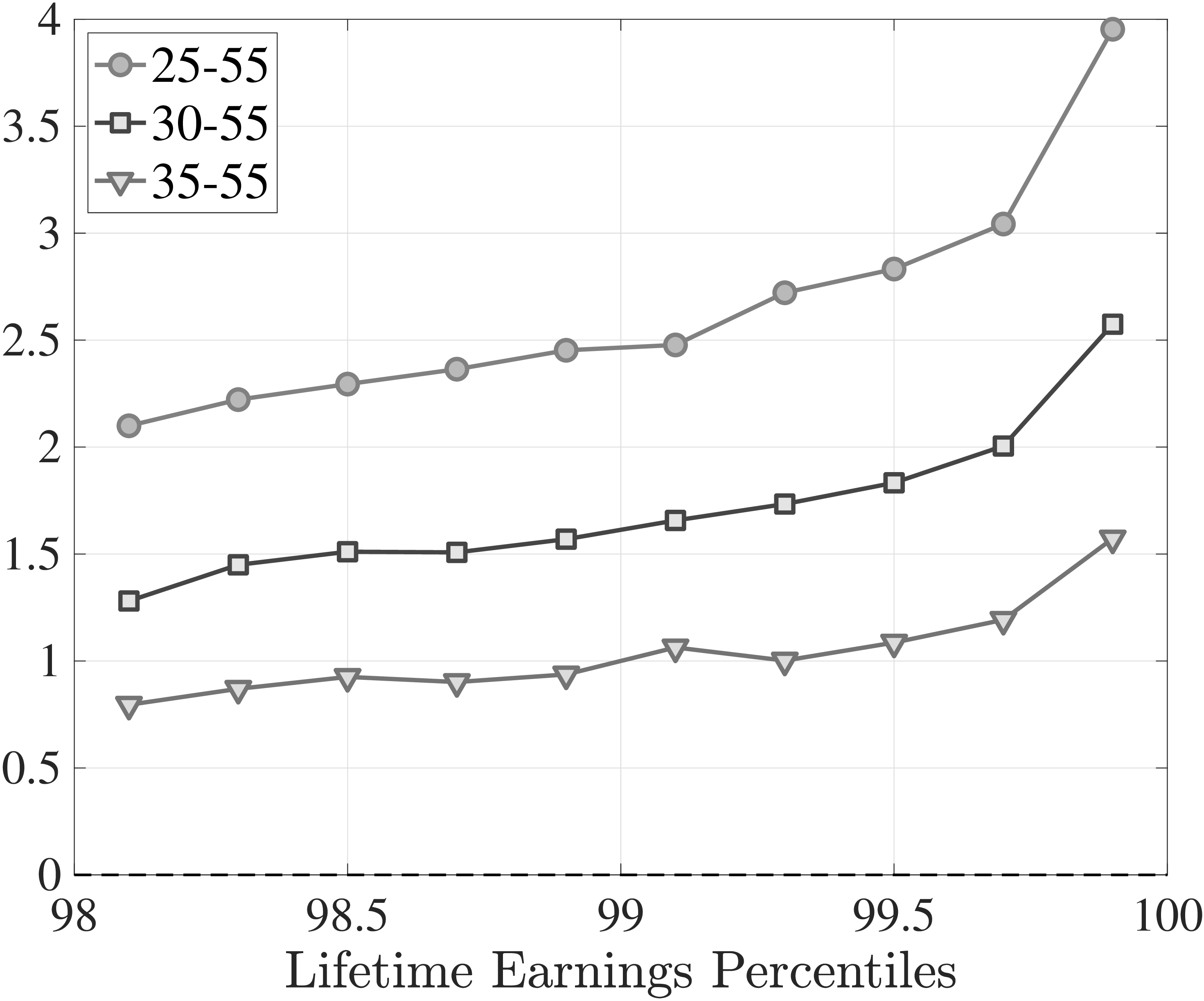
Notes: The left panel shows the average annual earnings over the life cycle for each LE group. The right panel shows the log difference of average earnings \(\bar{Y}\) between age 55 and various ages over the LE distribution.
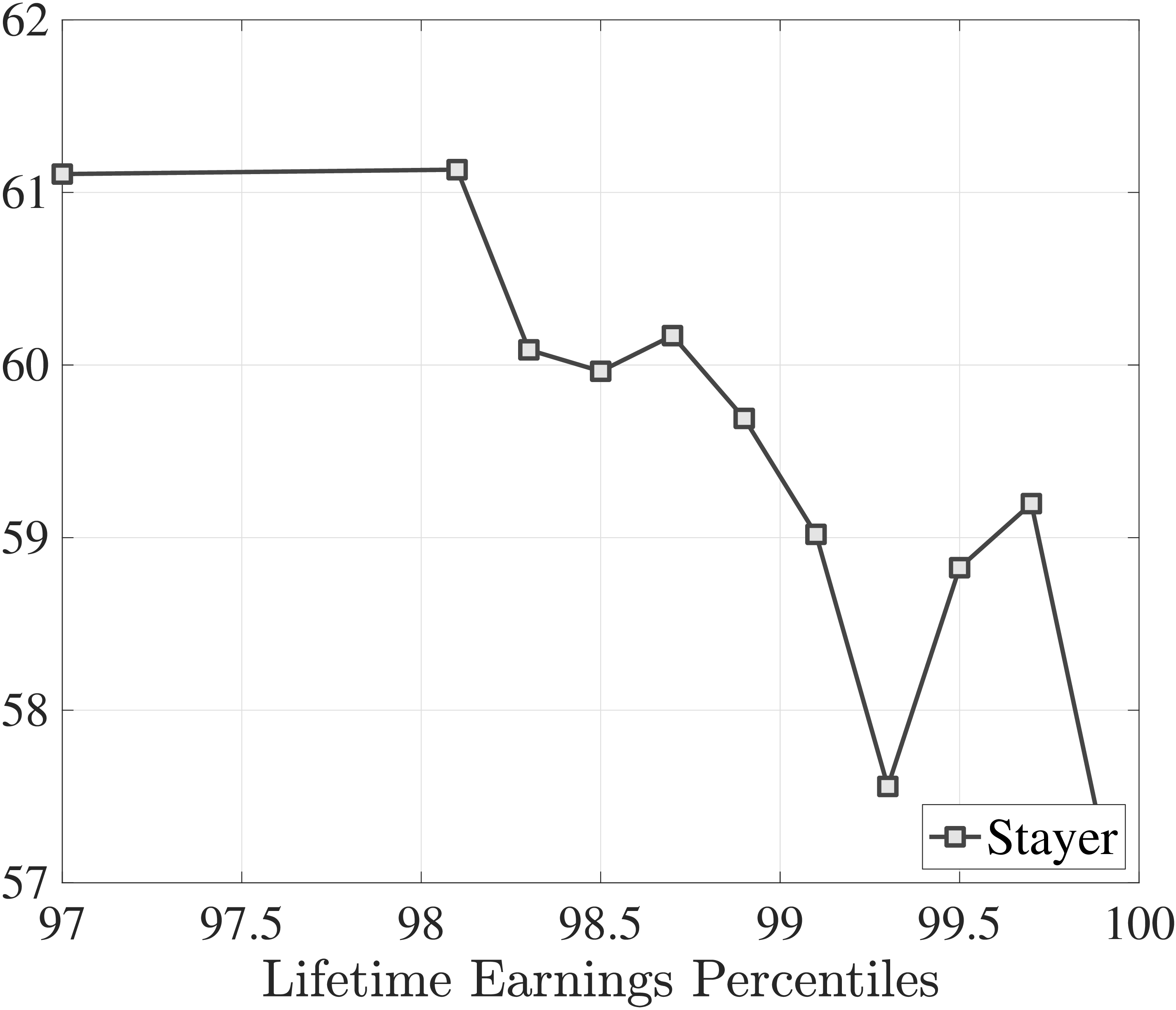
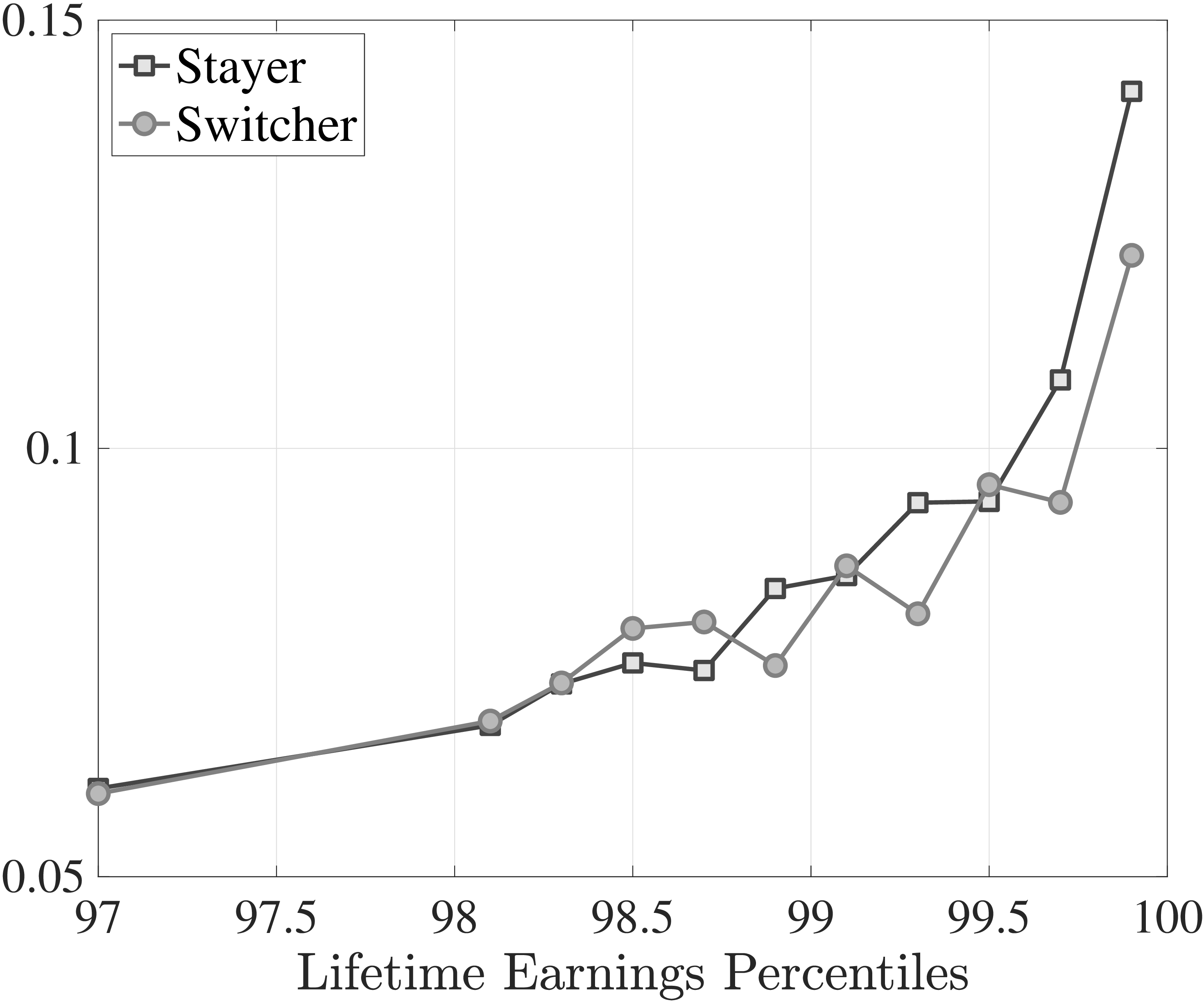
Notes: The left panel shows the fraction of workers in each LE group who are job stayers according to our definition, calculated for each age and averaged over the working life. The right panel plots the log growth of average earnings \(\bar{Y}\) between \(t\) and \(t+1\) for job stayers and switchers separately, again, averaged over \(t\) over the working life.
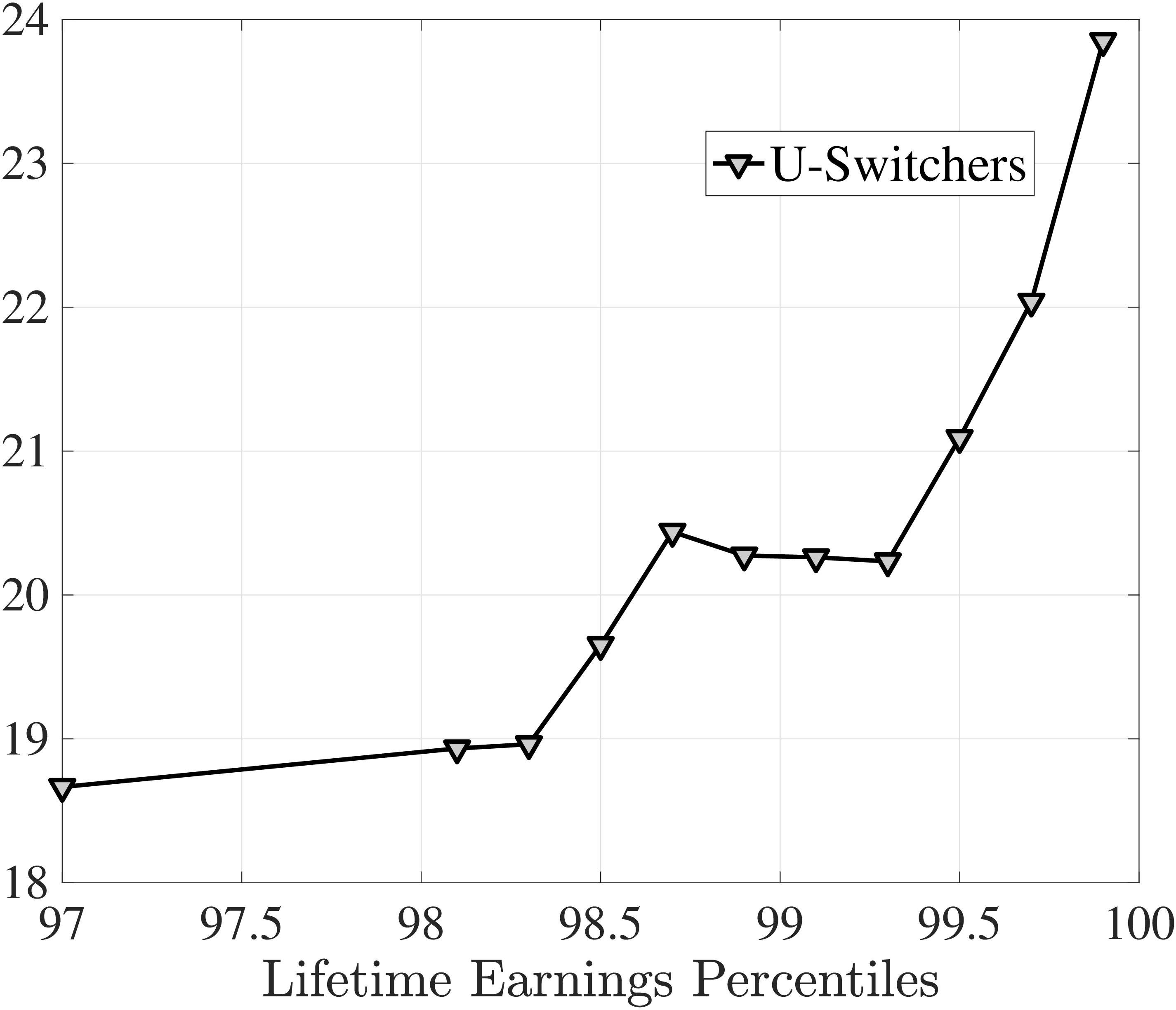
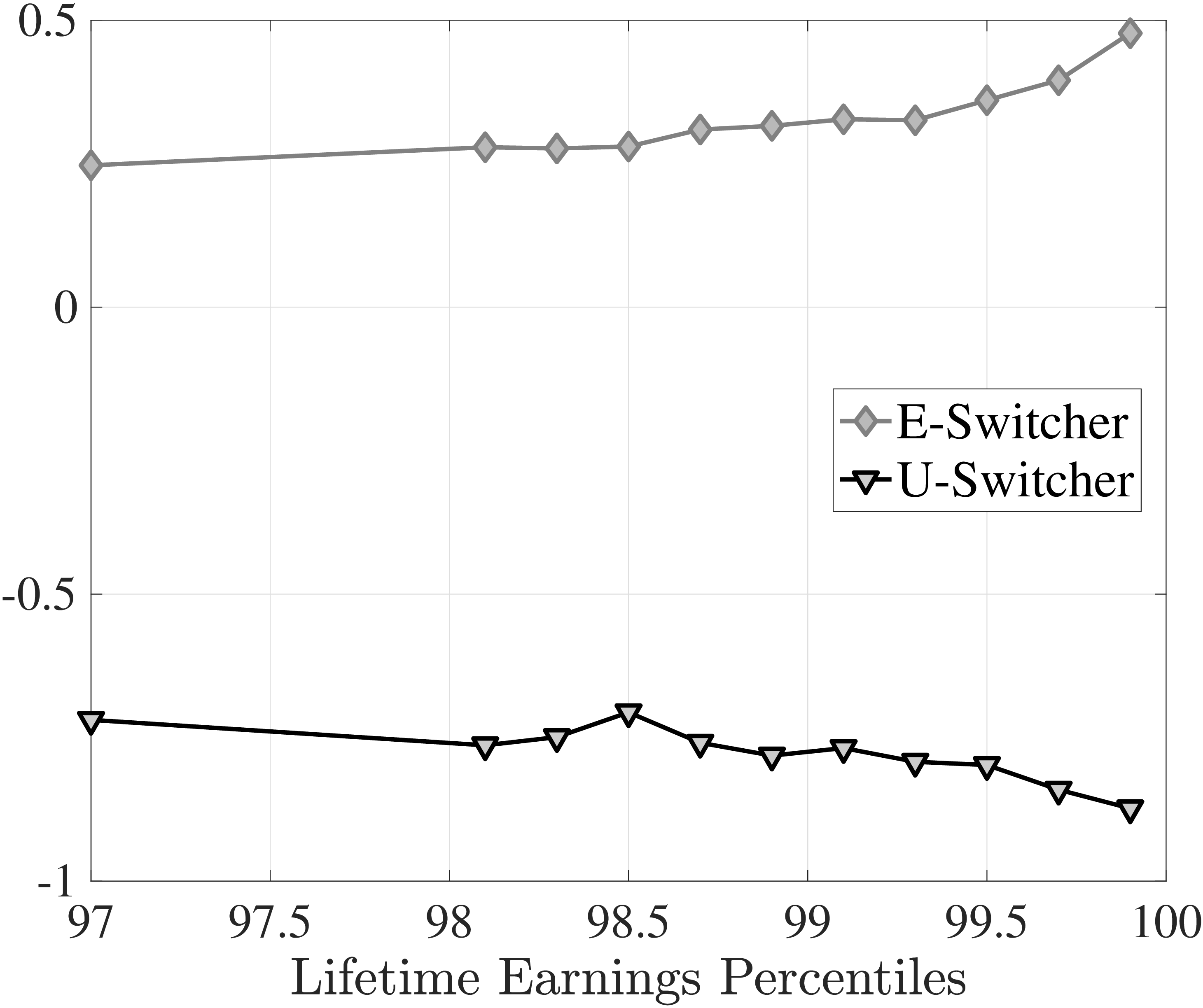
Notes: The left panel shows the share of U-switchers among job stayers in each LE group. The right panel plots the log growth of average earnings \(\bar{Y}\) between \(t\) and \(t+1\) for U-switchers and E-switchers separately.
8.3 Life cycle variation in switcher growth
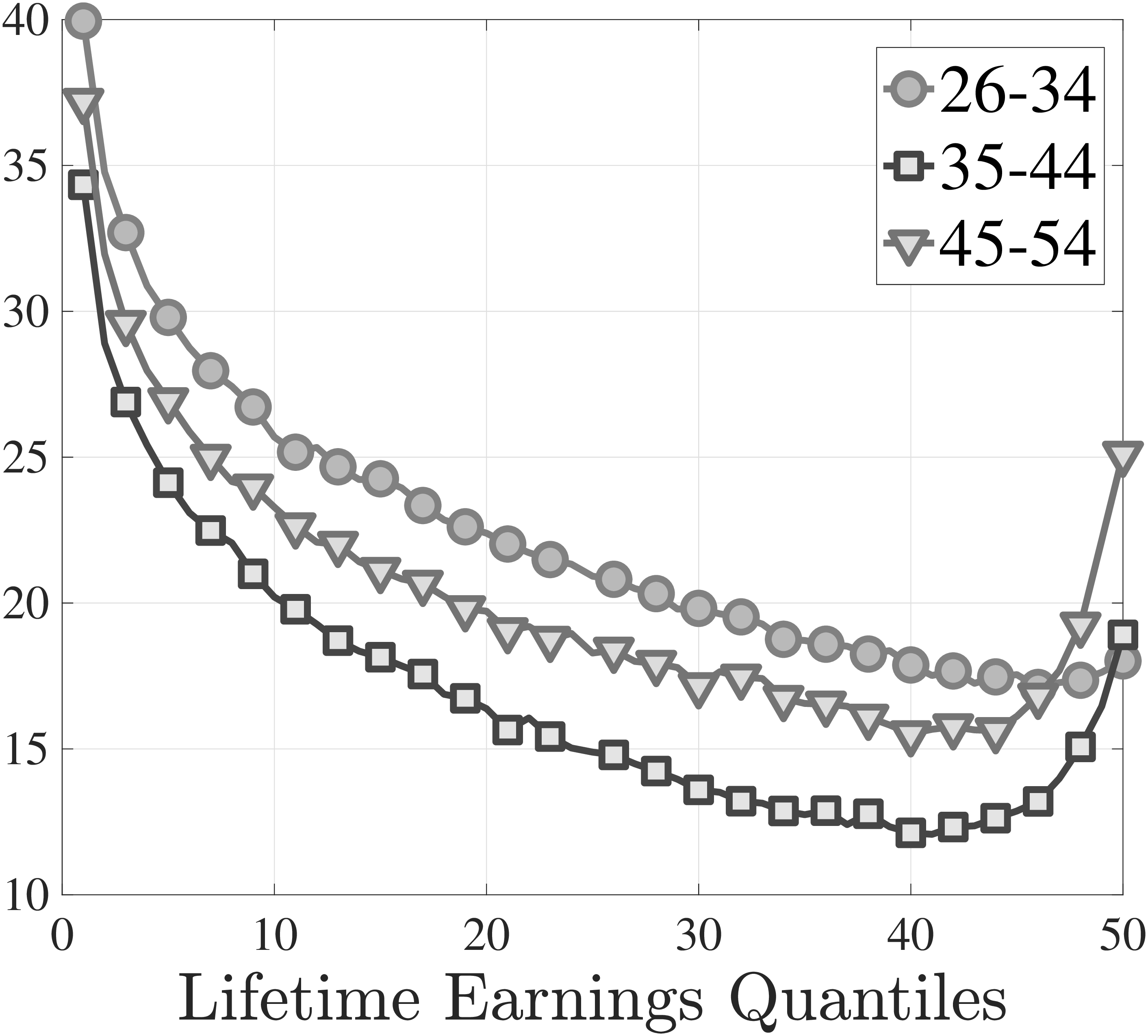
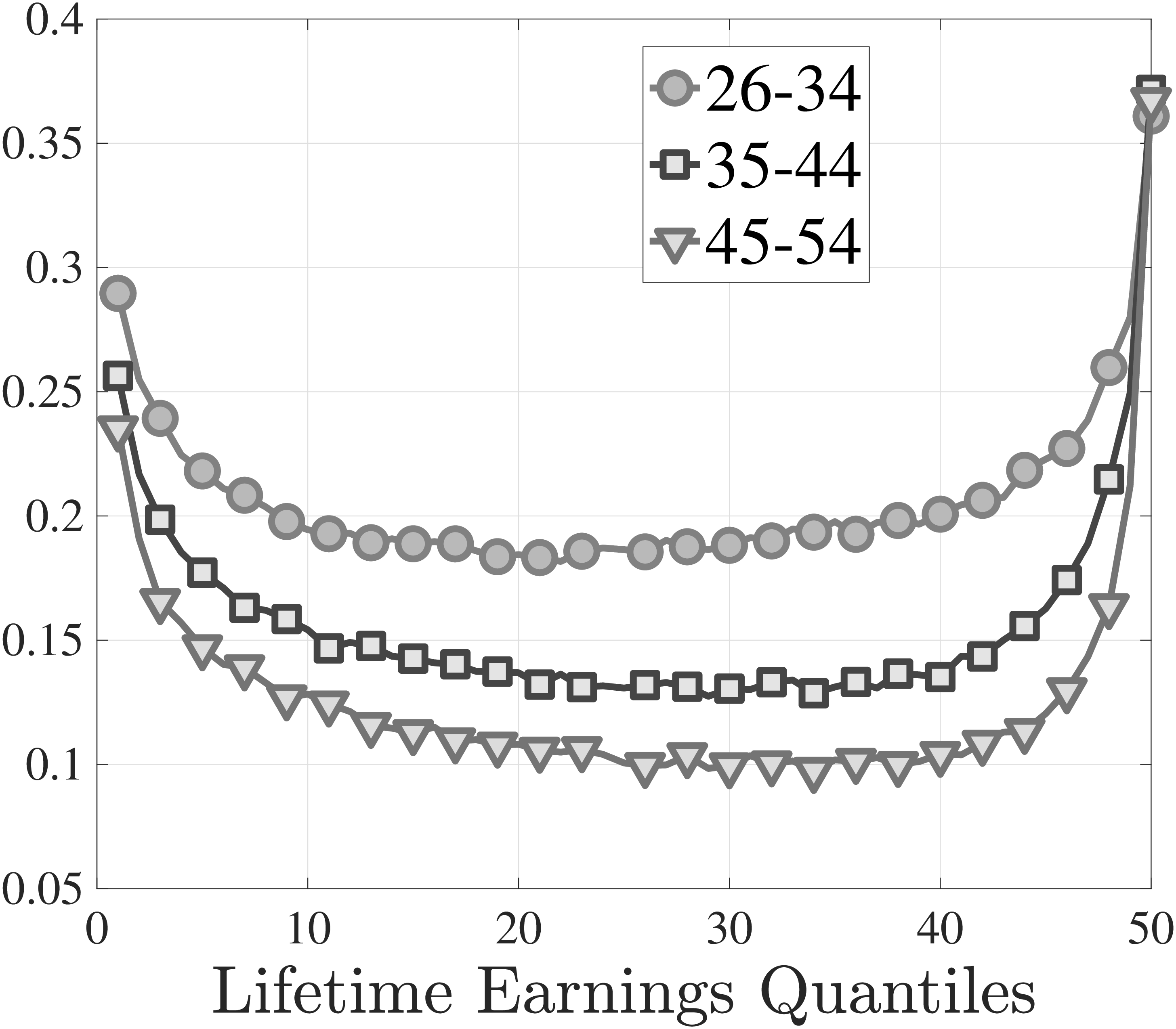
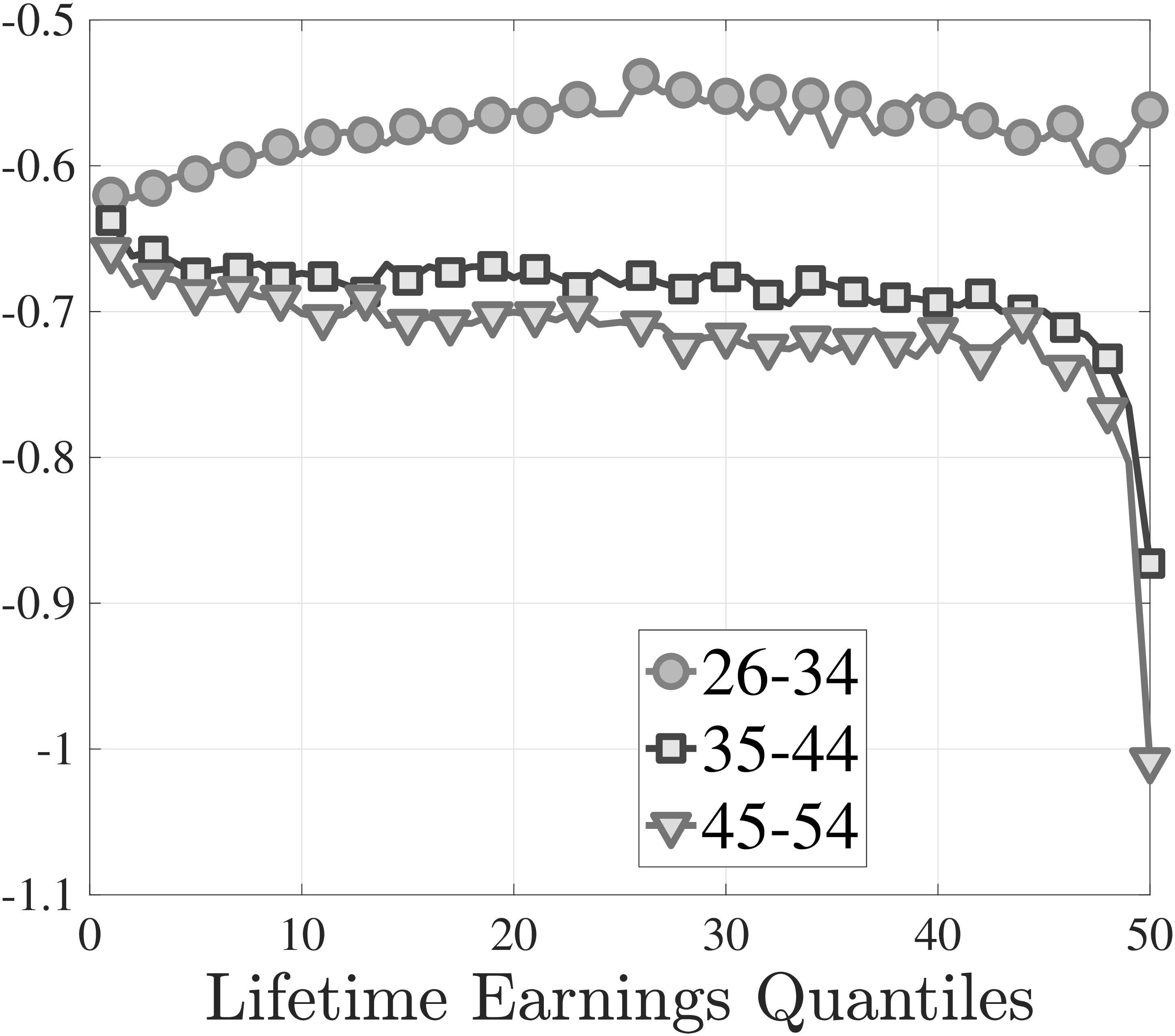
8.4 Moments for a Broader Sample
We select individuals for whom we have 33 years of data between ages 25 and 60 over 1978 and 2013. Furthermore, we exclude individuals who do not have earnings above the time-varying minimum earnings threshold for at least 15 years or who are self-employed for more than 8 years over their life cycle.
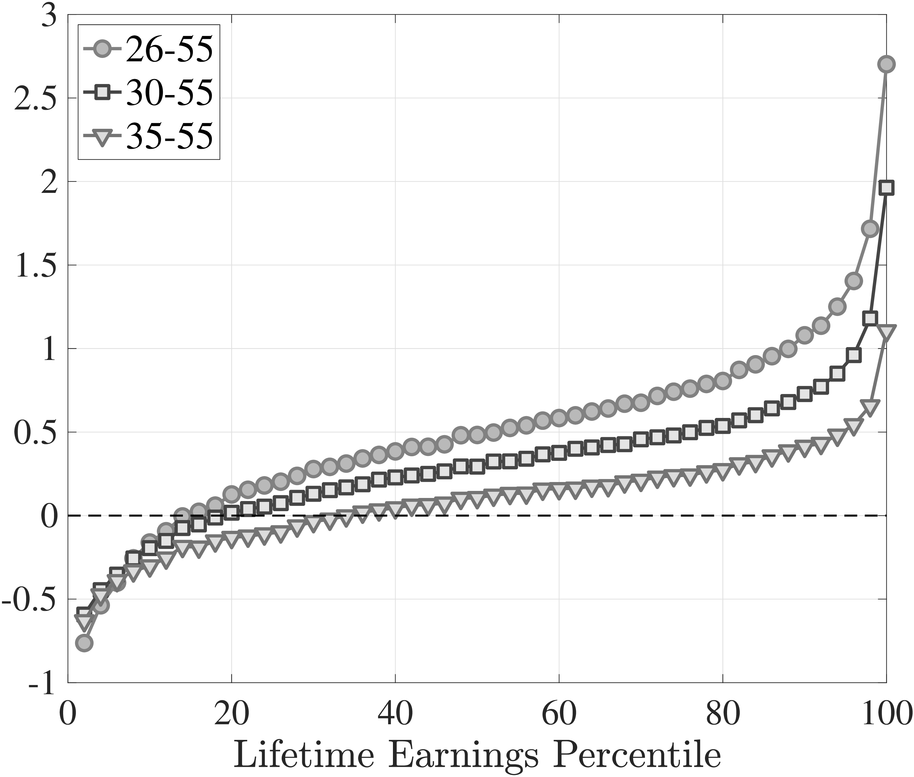
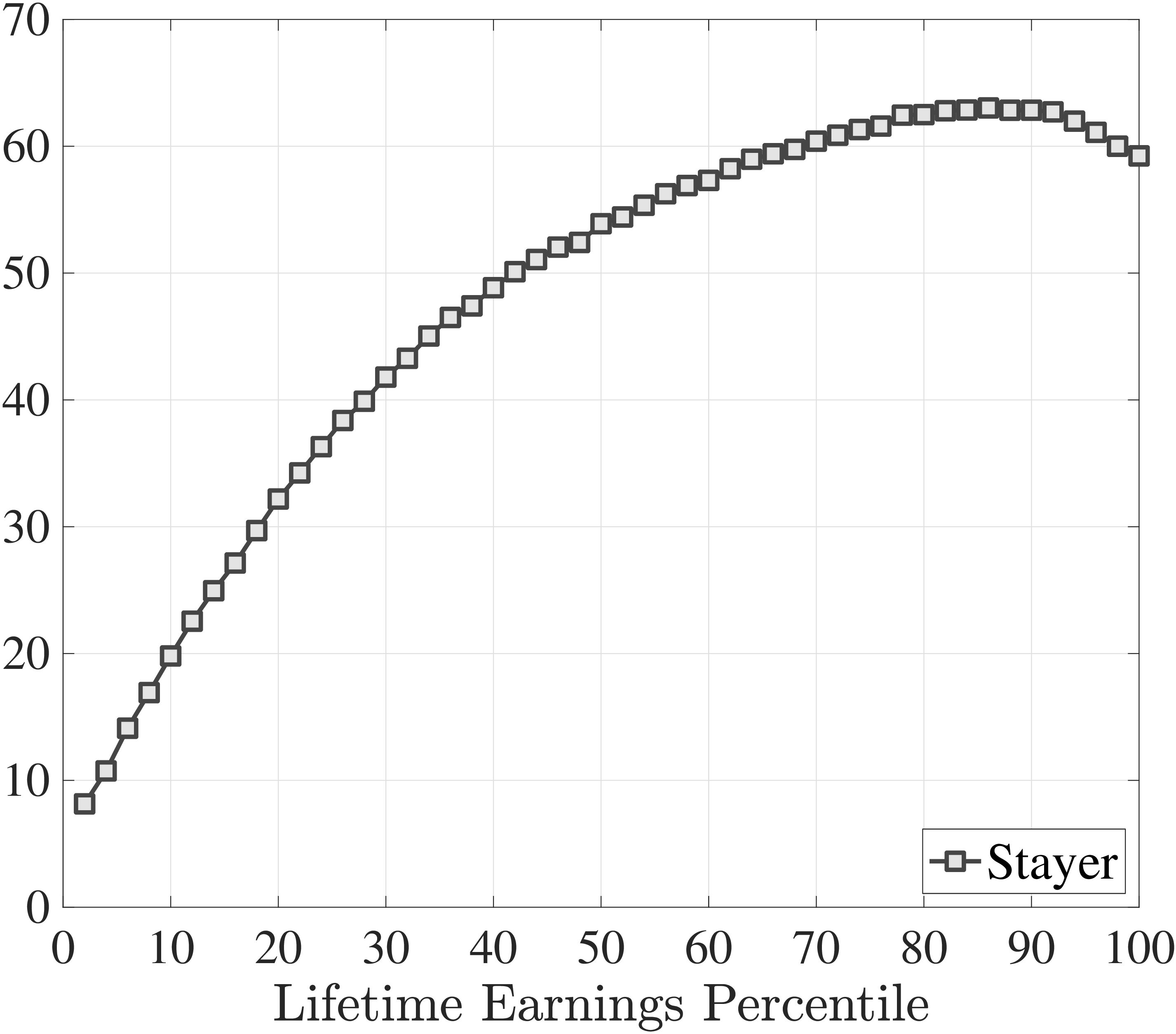
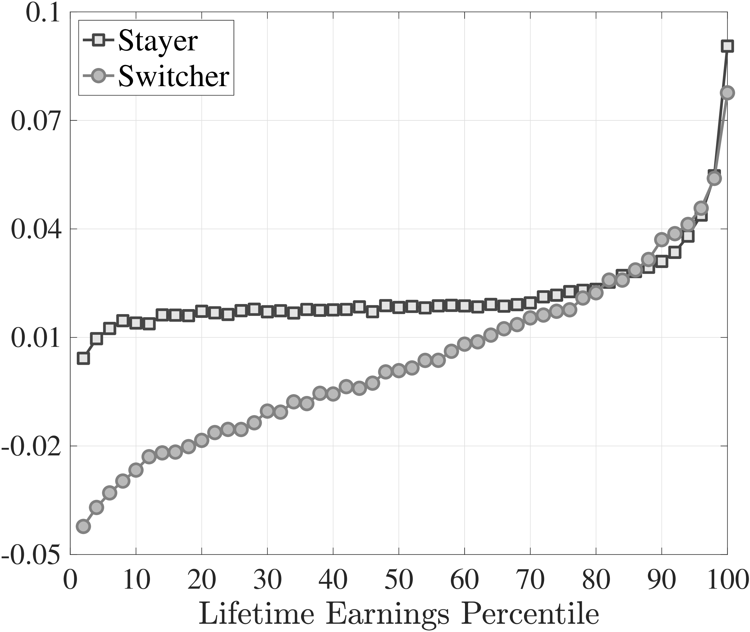
8.5 Earnings Growth Using Full-Year Employment
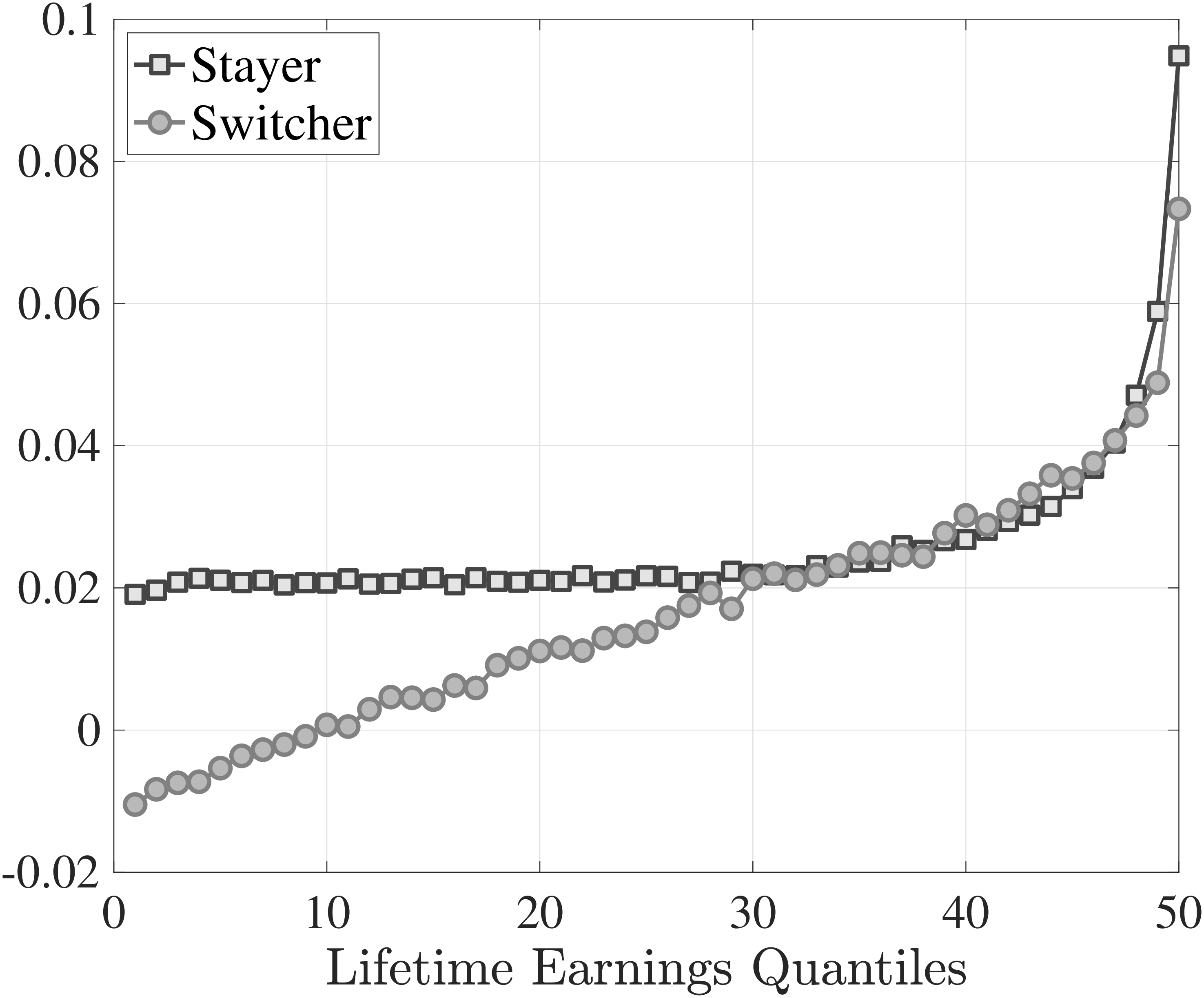
![(b) Average log growth, $\mathbb{E}\left [y_{t+1}-y_{t}\right]$](FINAL_SUBM_assets/FY_AvgLogWageGrwth_Inc2G_26to47-011b536d98.png)
Notes: The left panel shows the fraction of workers in each LE group who are job stayers according to our definition, calculated for each age and averaged over the working life. The right panel plots the log growth of average earnings \(\bar{Y}\) between \(t\) and \(t+1\) for job stayers and switchers separately, again, averaged over \(t\) over the working life.
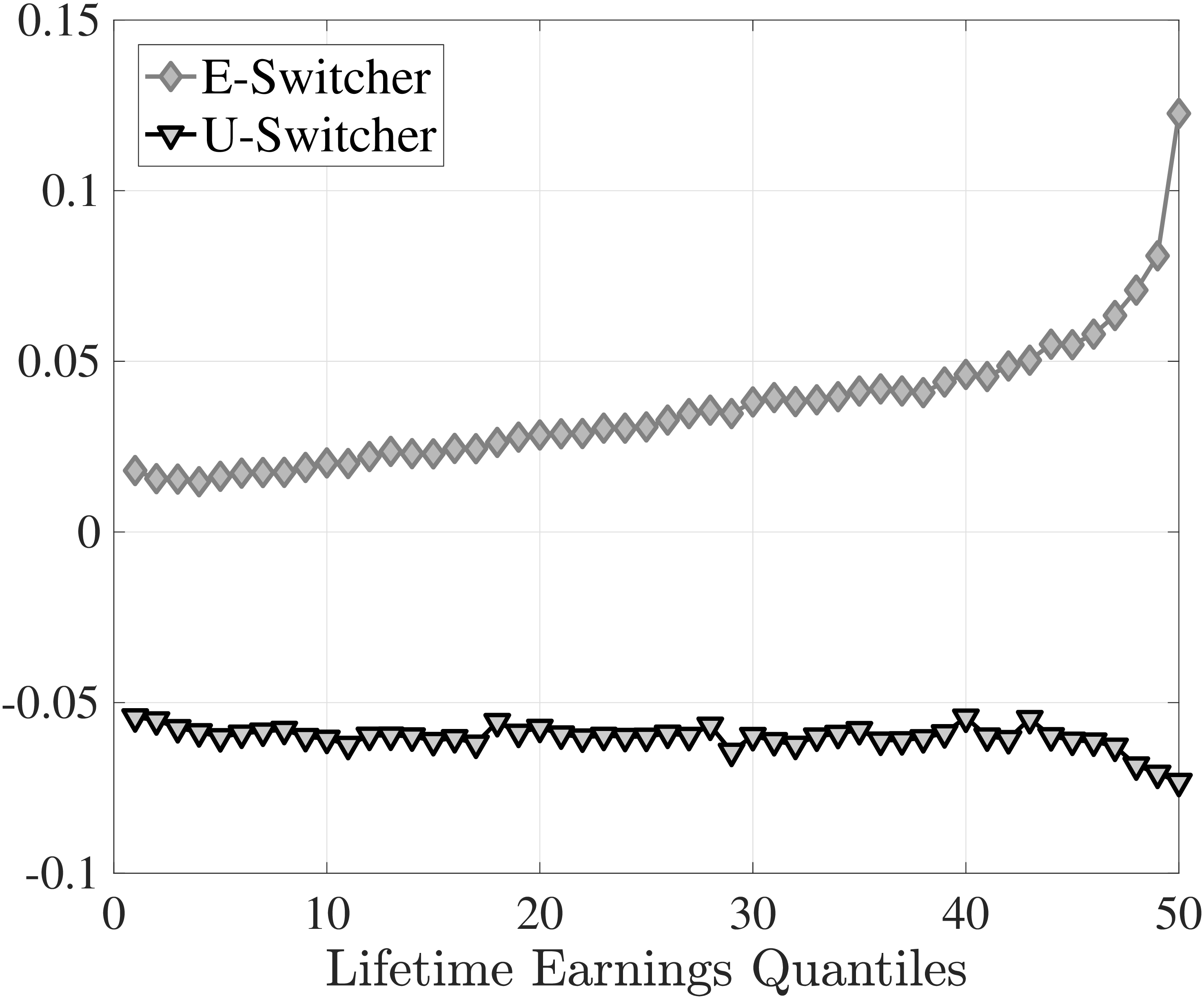
![(b) Average log growth, $\mathbb{E}\left [y_{t+1}-y_{t}\right]$](FINAL_SUBM_assets/FY_AvgLogWageGrwth_2G_NonStay_26to47-e7b3a0e065.png)
Notes: The left panel shows the share of U-switchers among job stayers in each LE group. The right panel plots the log growth of average earnings \(\bar{Y}\) between \(t\) and \(t+1\) for U-switchers and E-switchers separately.
9 Survey of Income and Program Participation
There are two important drawbacks to the SSA data. The first is their annual frequency, which doesn’t allow us to see higher frequency movements in earnings. The second is that they do not allow us to condition the outcomes on the labor market status of workers. To supplement the facts documented in the previous section, we use data from the Survey of Income and Program Participation (SIPP), a nationally representative sample of U.S. households. The data consist of monthly observations in overlapping panels with length between 2.5 and 4 years, with the first panel conducted in 1984. Each SIPP panel is conducted in waves, interviewing households every four months about the prior four months. Using data on labor force status, employment rates and labor market transition rates can be computed at a monthly frequency from the SIPP. Similarly, using individual income data, we are able to investigate how these flow rates vary with the level of earnings.39 We also use the SIPP to compute labor market flow rates for individuals by educational attainment.
9.1 Sample
The SIPP sample is selected in a way that mirrors (to the extent possible) the SSA sample construction. We select males between the ages of 25 and 55. We convert nominal monthly wage data to real using the personal consumption expenditure (PCE) deflator, using 2010 as the base year. We require people to have prior data for at least 36 months and construct their previous income, by summing their monthly real wage over the past 32 months. We residualize this past income by regressing its logarithm on a full set of age and year dummies. We assign individuals into deciles based on this residual.
9.2 Heterogeneity in Labor Market Flows
We compute rates of three types of labor market flows, EU, UE and EE, over a four-month period to deal with seam bias documented in previous work. Observations that report UNU or NUN over three consecutive months are recoded as UUU and NNN, respectively. We use the employer ID to construct job-to-job transitions. We rank workers into 10 equally sized deciles within each age group (25–34, 35–44 and 45–55) based on their recent earnings (RE) over the past three years. Next, we compute the job loss (EU), job finding (UE), and job-to-job (EE) transition rates for each group over the next four months.
Job loss rates show significant heterogeneity across previous recent earnings deciles for all age groups (Figure B.1). For example, unemployment risk at the bottom decile can be almost five times that of the top decile. There are also marked differences over the life cycle, with young workers much more exposed to unemployment than older ones. Our finding indicates that workers with low wages are more likely to fall of the job ladder, and would arguably therefore not be able to move to better jobs, as that requires clinging on to the job ladder. Earlier literature has emphasized the life-cycle variation in unemployment risk (Jung and Kuhn (2018); Shimer (2001)). We find that between-RE variation in job loss rates is an order of magnitude larger. The middle panel shows that the four-month job finding probabilities (UE rates) are strongly increasing with the level of past earnings. This rate is around 30% for young workers (25-34) with low earnings, and increases monotonically up to 90%. Moving to job-to-job transition rates (right panel), we find that over a four-month period these are as high as 10% for young workers with low earnings, decline with recent earnings, and are about 4% for the top decile—as we discuss in Section 5, a feature of the data our model can replicate as well.
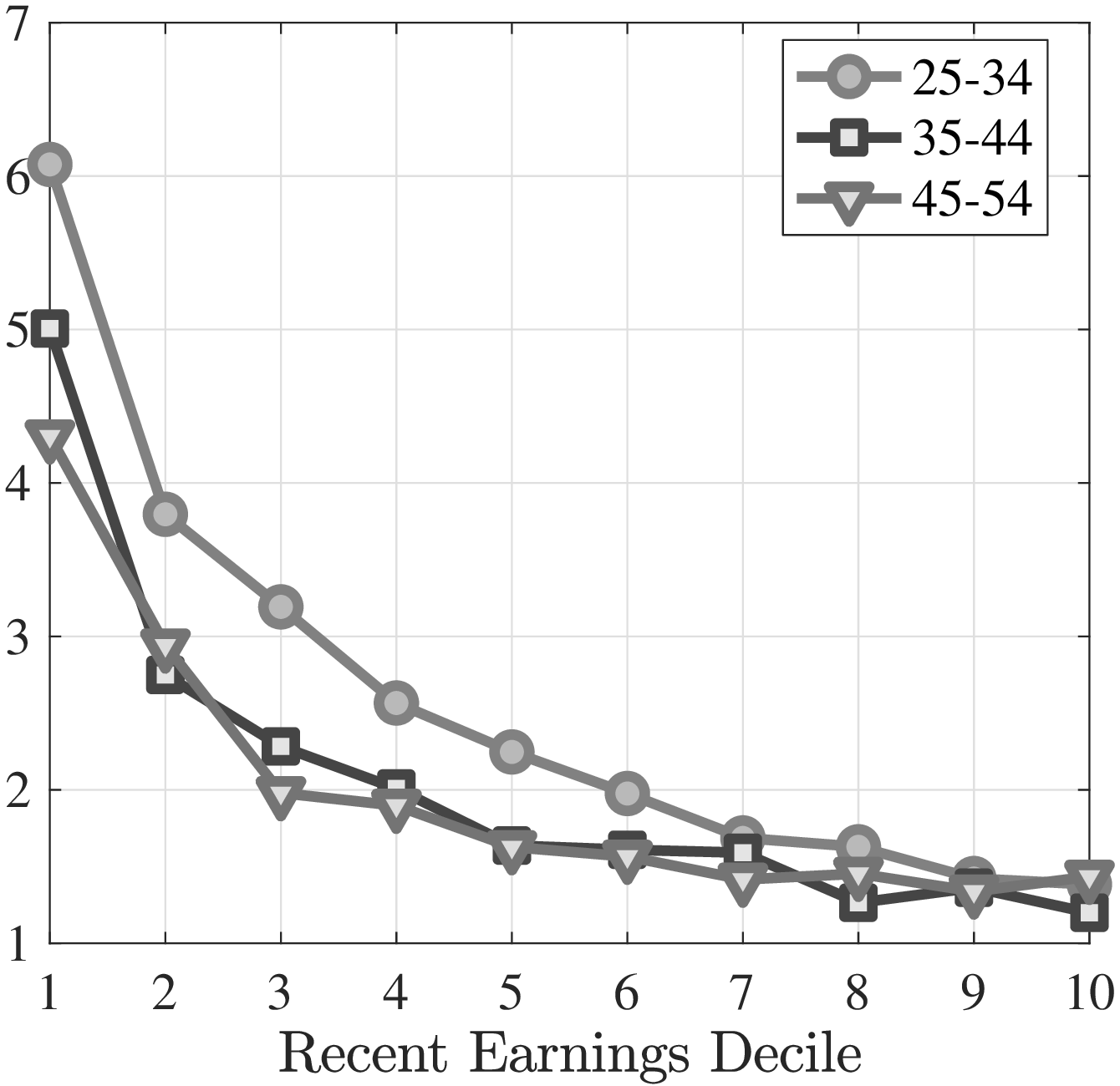
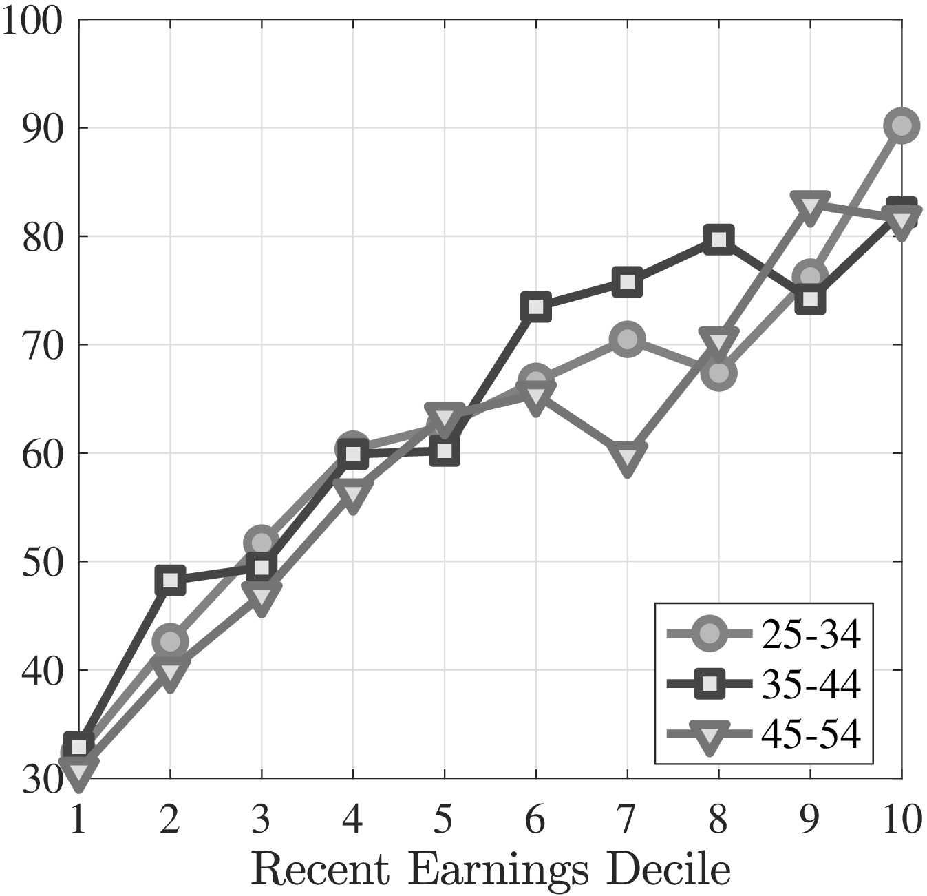
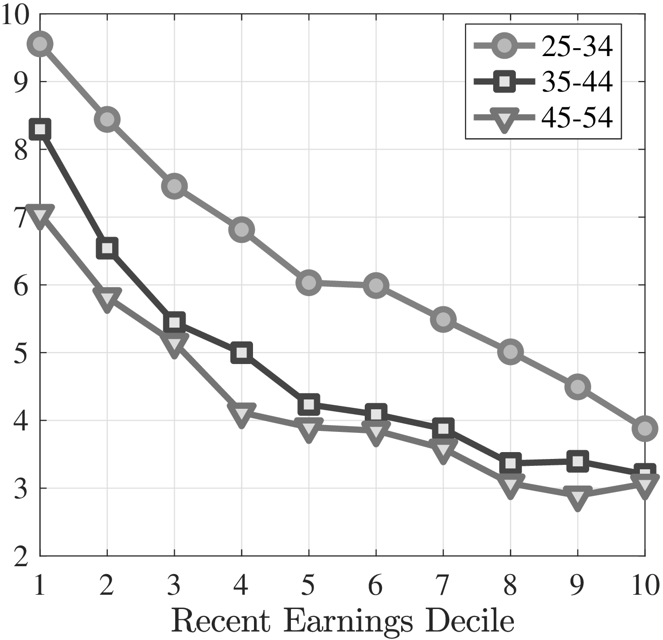
10 Model Derivations
To the baseline model in Bagger et al. (2014), we add a recall option and stochastic aging. Let \(\lambda _{r}\) denote the probability of recall for unemployed workers. The superscripts \(y\) and \(o\) refer to young and old workers, respectively. Young workers become old with probability \(\gamma\). We start by deriving the wage equation for old workers and proceed backwards to solve the same for young workers. These derivations follow closely those in Bagger et al. (2014).
Solving piece rates for old workers
Let \(V^{o}\left (r,h,p\right)\) denote the value function of an old worker with human capital \(h\) employed at a firm with productivity \(p\) at (log-) piece rate \(r\). Note that we are suppressing the dependence of the value functions and labor market transitions (\(\delta\), \(\lambda _{0}\), \(\lambda _{1}\)) on individual ability \(\alpha _{i}\) and return to experience \(\beta _{i}\). For ease of notation, we also suppress the functional form for wages (\(w=r+p+h\)). Finally, we let \(\kappa ^{o}=\xi \lambda _{0}^{o}\) and \(\kappa ^{y}=\xi \lambda _{0}^{y}\) denote the rate at which workers that lose their job in a period find another job immediately within the same period. \(V^{o}\left (r,h,p\right)\) is given by
\[ \begin{aligned} V^{o}\left (r,h,p\right) & = & w+\frac{\delta ^{o}\left (1-\kappa ^{o}\right)}{1+\rho}V_{0}^{o}\left (h\right)+\frac{\kappa ^{o}}{1+\rho}\int _{p}^{\bar{p}}\mathbb{E}\left [\left (1-\theta \right)V_{0}\left (h\right)+\theta V^{o}\left (0,h',x\right)\right]dF\left (x\right) \\ & & +\frac{\lambda _{1}^{o}}{1+\rho}\int _{p}^{\bar{p}}\mathbb{E}\left [\left (1-\theta \right)V^{o}\left (0,h',p\right)+\theta V^{o}\left (0,h',x\right)\right]dF\left (x\right) \\ & & +\frac{\lambda _{1}^{o}}{1+\rho}\int _{q^{o}\left (r,h,p\right)}^{p}\mathbb{E}\left [\left (1-\theta \right)V^{o}\left (0,h',x\right)+\theta V^{o}\left (0,h',p\right)\right]dF\left (x\right) \\ & & +\frac{1}{1+\rho}\left [1-\delta ^{o}-\lambda _{1}^{o}\bar{F}\left (q^{o}\left (r,h,p\right)\right)\right]\mathbb{E}V^{o}\left (r,h',p\right). \end{aligned} \]
Integrating (3) by parts, we obtain
\[ \begin{aligned} V^{o}\left (r,h,p\right) & = & w+\frac{\delta ^{o}}{1+\rho}V_{0}^{o}\left (h\right)+\frac{1}{1+\rho}\mathbb{E}\bigg \{\left (1-\delta ^{o}\right)V^{o}\left (r,h',p\right) \\ & & +\lambda _{1}^{o}\theta \int _{p}^{\bar{p}}\frac{\partial V^{o}}{\partial x}\left (0,h',x\right)\bar{F}\left (x\right)dx \\ & & +\lambda _{1}^{o}\left (1-\theta \right)\int _{q^{o}\left (r,h,p\right)}^{p}\frac{\partial V^{o}}{\partial x}\left (0,h',x\right)\bar{F}\left (x\right)dx \\ & & +\delta \kappa ^{o}\theta \int _{p_{\text{min}}}^{\bar{p}}\frac{\partial V^{o}}{\partial x}\left (0,h',x\right)\bar{F}\left (x\right)dx\bigg \} \end{aligned} \]
Applying (4) with \(r=0\), and noting that \(q\left (0,h,p\right)=p\), we get \[\begin{aligned} V^{o}\left (0,h,p\right) &= p+h+\frac{\delta ^{o}}{1+\rho}V_{0}^{o}\left (h\right)+\frac{1}{1+\rho}\mathbb{E}\bigg \{\left (1-\delta ^{o}\right)V^{o}\left (0,h',p\right)\\ & +\lambda _{1}^{o}\beta \int _{p}^{\bar{p}}\frac{\partial V^{o}}{\partial x}\left (0,h',x\right)\bar{F}\left (x\right)dx\\ & +\delta \kappa ^{o}\theta \int _{p_{\text{min}}}^{\bar{p}}\frac{\partial V^{o}}{\partial x}\left (0,h',x\right)\bar{F}\left (x\right)dx\bigg \} \end{aligned}\] Then, we differentiate this expression with respect to \(p\), to obtain: \[\begin{aligned} \frac{\partial V^{o}}{\partial p}\left (0,h,p\right) &= 1+\left [\frac{1-\delta ^{o}-\lambda _{1}^{o}\theta \bar{F}\left (p\right)}{1+\rho}\right]\frac{\partial V^{o}}{\partial p}\left (0,h',p\right). \end{aligned}\]
This expression, upon collecting terms yields \[ \frac{\partial V^{o}}{\partial p}\left (0,h,p\right)=\frac{1+\rho}{\rho +\delta ^{o}+\lambda _{1}^{o}\theta \bar{F}\left (p\right)}. \] Substituting this expression back in (4), and letting \(C^{o}\left (p\right)\equiv \frac{1}{\rho +\delta ^{o}+\lambda _{1}^{o}\theta \bar{F}\left (x\right)},\) we get
\[ \begin{aligned} V^{o}\left (r,h,p\right) & = & w+\frac{\delta ^{o}}{1+\rho}V_{0}^{o}\left (h\right) \\ & & +\frac{1}{1+\rho}\mathbb{E}\bigg \{\left (1-\delta ^{o}\right)V^{o}\left (r,h',p\right) \\ & & +\lambda _{1}^{o}\theta \int _{p}^{\bar{p}}\left (1+\rho \right)C^{o}\left (x\right)\bar{F}\left (x\right)dx \\ & & +\lambda _{1}^{o}\left (1-\theta \right)\int _{q^{o}\left (r,h,p\right)}^{p}\left (1+\rho \right)C^{o}\left (x\right)\bar{F}\left (x\right)dx \\ & & +\delta \kappa ^{o}\theta \int _{p_{\text{min}}}^{\bar{p}}\left (1+\rho \right)C^{o}\left (x\right)\bar{F}\left (x\right)dx\bigg \} \end{aligned} \]
Note that \(q^{o}\) is defined by the following indifference condition:
\[ \mathbb{E}V^{o}\left (r,h',p\right)=\mathbb{E}\left \{V^{o}\left (0,h',q^{o}\right)+\theta \left [V^{o}\left (0,h',p\right)-V^{o}\left (0,h',q^{o}\right)\right]\right \} \]
We first rewrite this as follows: \[ \mathbb{E}V^{o}\left (r,h',p\right)-V^{o}\left (0,h',q^{o}\right)=\theta \mathbb{E}\left \{V^{o}\left (0,h',p\right)-V^{o}\left (0,h',q^{o}\right)\right \} \] Substituting (5) into this, and rearranging terms, we obtain
\[ \begin{aligned} r+p-q^{o}\left (r,h,p\right)+\frac{1-\delta ^{o}}{1+\rho}\left [V^{o}\left (r,h'',p\right)-V^{o}\left (0,h'',q^{o}\right)\right]\\ -\lambda _{1}^{o}\theta \int _{q^{o}}^{p}\frac{\left (1+\rho \right)\bar{F}\left (x\right)}{\rho +\delta ^{o}+\lambda _{1}^{o}\theta \bar{F}\left (x\right)}dx+\frac{\lambda _{1}^{o}\left (1-\theta \right)}{1+\rho}\int _{q^{o}\left (r,h,p\right)}^{p}\frac{\left (1+\rho \right)\bar{F}\left (x\right)}{\rho +\delta ^{o}+\lambda _{1}^{o}\theta \bar{F}\left (x\right)}dx & =\\ \mathbb{E}\bigg \{\theta \left [p-q^{o}\left (r,h,p\right)\right]+\theta \frac{1-\delta ^{o}}{1+\rho}\left [V^{o}\left (0,h'',p\right)-V^{o}\left (0,h'',q^{o}\right)\right]\bigg \}\\ -\lambda _{1}^{o}\theta ^{2}\int _{q^{o}}^{p}\frac{\left (1+\rho \right)\bar{F}\left (x\right)}{\rho +\delta ^{o}+\lambda _{1}^{o}\theta \bar{F}\left (x\right)}dx \end{aligned} \]
Rearranging terms, we obtain \[\begin{aligned} r &= -\left (1-\theta \right)\left [p-q^{o}\left (r,h,p\right)\right]-\lambda _{1}^{o}\left (1-\theta \right)^{2}\int _{q\left (r,h,p\right)}^{p}\frac{\left (1+\rho \right)\bar{F}\left (x\right)dx}{\rho +\delta ^{o}+\lambda _{1}^{o}\theta \bar{F}\left (x\right)}\\ & +\frac{1-\delta ^{o}}{1+\rho}\mathbb{E}\left [\left (1-\theta \right)V^{o}\left (0,h'',q\left (r,h_{t},p\right)\right)+\theta V^{o}\left (0,h'',p\right)-V^{o}\left (r,h'',p\right)\right] \end{aligned}\] Substituting the last term with (6) and using the law of iterated expectations, we get \[\begin{aligned} r &= -\left (1-\theta \right)\left [p-q^{o}\left (r,h,p\right)\right]-\lambda _{1}^{o}\left (1-\theta \right)^{2}\int _{q\left (r,h,p\right)}^{p}\frac{\left (1+\rho \right)\bar{F}\left (x\right)dx}{\rho +\delta ^{o}+\lambda _{1}^{o}\theta \bar{F}\left (x\right)}\\ & +\frac{\left (1-\delta ^{o}\right)\left (1-\theta \right)}{1+\rho}\mathbb{E}\left [V^{o}\left (0,h'',q^{o}\left (r,h,p\right)\right)-V^{o}\left (0,h'',q^{o}\left (r,h',p\right)\right)\right]\\ &= -\left (1-\theta \right)\left [p-q^{o}\left (r,h,p\right)\right]-\lambda _{1}^{o}\left (1-\theta \right)^{2}\int _{q^{o}\left (r,h,p\right)}^{p}\frac{\bar{F}\left (x\right)dx}{\rho +\delta ^{o}+\lambda _{1}^{o}\theta \bar{F}\left (x\right)}\\ & -\frac{\left (1-\delta ^{o}\right)\left (1-\theta \right)}{1+\rho}\mathbb{E}\int _{q^{o}\left (r,h,p\right)}^{q^{o}\left (r,h',p\right)}\frac{\partial V^{o}}{\partial p}\left (0,h'',x\right)dx\\ &= -\left (1-\theta \right)\left [p-q^{o}\left (r,h,p\right)\right]-\lambda _{1}^{o}\left (1-\theta \right)^{2}\int _{q^{o}\left (r,h,p\right)}^{p}\frac{\bar{F}\left (x\right)dx}{\rho +\delta ^{o}+\lambda _{1}^{o}\theta \bar{F}\left (x\right)}\\ & -\frac{\left (1-\delta ^{o}\right)\left (1-\theta \right)}{1+\rho}\mathbb{E}\int _{q^{o}\left (r,h,p\right)}^{q^{o}\left (r,h',p\right)}\frac{dx}{\rho +\delta ^{o}+\lambda _{1}^{o}\theta \bar{F}\left (x\right)}. \end{aligned}\]We look for a deterministic solution (constant with respect to \(h\)). This solution is implicitly defined by r=-(1-)-{1}^{o}(1-)^{2}{q^{o}(r,p)}{p}C{o}(x){F}(x)dx
Solving piece rates for young workers
The value function for young workers is as follows:
\[ \begin{aligned} V^{y}\left (r,h,p\right) & = & w+\frac{\delta ^{y}(1-\kappa ^{y})}{1+\rho}V_{0}^{y}\left (h\right) \\ & & +\frac{\kappa ^{y}}{1+\rho}\int _{p}^{\bar{p}}\mathbb{E}\left [\left (1-\theta \right)V_{0}\left (h\right)+\theta V^{y}\left (0,h',x\right)\right]dF\left (x\right) \\ & & +\frac{\lambda _{1}^{y}}{1+\rho}\int _{p}^{\bar{p}}\mathbb{E}\left [\left (1-\theta \right)V^{y}\left (0,h',p\right)+\theta V^{y}\left (0,h',x\right)\right]dF\left (x\right) \\ & & +\frac{\lambda _{1}^{y}}{1+\rho}\int _{q^{y}\left (r,h,p\right)}^{p}\mathbb{E}\left [\left (1-\theta \right)V^{y}\left (0,h',x\right)+\theta V^{y}\left (0,h',p\right)\right]dF\left (x\right) \\ & & +\frac{\gamma}{1+\rho}\mathbb{E}V^{o}\left (r,h',p\right) \\ & & +\frac{1}{1+\rho}\left [1-\delta ^{y}-\gamma -\lambda _{1}^{y}\bar{F}\left (q^{y}\left (r,h,p\right)\right)\right]EV^{y}\left (r,h',p\right) \end{aligned} \]
Integrating (7) by parts, we obtain
\[ \begin{aligned} V^{y}\left (r,h,p\right) & = & w+\frac{\delta ^{y}}{1+\rho}V_{0}^{y}\left (h\right)+\frac{1}{1+\rho}\mathbb{E}\bigg \{\left (1-\delta ^{y}-\gamma \right)V^{y}\left (r,h',p\right) \\ & & +\lambda _{1}^{y}\theta \int _{p}^{\bar{p}}\frac{\partial V^{y}}{\partial x}\left (0,h',x\right)\bar{F}\left (x\right)dx \\ & & +\lambda _{1}^{y}\left (1-\theta \right)\int _{q^{y}\left (r,h,p\right)}^{p}\frac{\partial V^{y}}{\partial x}\left (0,h',x\right)\bar{F}\left (x\right)dx \\ & & +\delta \kappa ^{y}\theta \int _{p_{\text{min}}}^{\bar{p}}\frac{\partial V^{y}}{\partial x}\left (0,h',x\right)\bar{F}\left (x\right)dx+\gamma \mathbb{E}V^{o}\left (r,h',p\right)\bigg \} \end{aligned} \]
Substituting the expression for \(V^{o}\) we derived earlier, we get
\[ \begin{aligned} V^{y}\left (r,h,p\right) & = & w+\frac{\delta ^{y}}{1+\rho}V_{0}^{y}\left (h\right)+\frac{1}{1+\rho}\mathbb{E}\bigg \{\left (1-\delta ^{y}-\gamma \right)V^{y}\left (r,h',p\right) \\ & & +\lambda _{1}^{y}\theta \int _{p}^{\bar{p}}\frac{\partial V^{y}}{\partial x}\left (0,h',x\right)\bar{F}\left (x\right)dx+\lambda _{1}^{y}\left (1-\theta \right)\int _{q^{y}\left (r,h,p\right)}^{p}\frac{\partial V^{y}}{\partial x}\left (0,h',x\right)\bar{F}\left (x\right)dx \\ & & +\delta \kappa ^{y}\theta \int _{p_{\text{min}}}^{\bar{p}}\frac{\partial V^{y}}{\partial x}\left (0,h',x\right)\bar{F}\left (x\right)dx \\ & & +\gamma \bigg (w'+\frac{\delta ^{o}}{1+\rho}V_{0}^{o}\left (h''\right)+\frac{1}{1+\rho}\bigg \{\left (1-\delta ^{o}\right)V^{o}\left (r,h'',p\right) \\ & & +\lambda _{1}^{o}\theta \int _{p}^{\bar{p}}\frac{\left (1+\rho \right)\bar{F}\left (x\right)}{\rho +\delta ^{o}+\lambda _{1}^{o}\theta \bar{F}\left (x\right)}dx+\lambda _{1}^{o}\left (1-\theta \right)\int _{q^{o}\left (r,h',p\right)}^{p}\frac{\left (1+\rho \right)\bar{F}\left (x\right)}{\rho +\delta ^{o}+\lambda _{1}^{o}\theta \bar{F}\left (x\right)}dx \\ & & +\delta \kappa ^{o}\theta \int _{p_{\text{min}}}^{\bar{p}}\frac{\left (1+\rho \right)}{\rho +\delta ^{o}+\lambda _{1}^{o}\theta \bar{F}\left (x\right)}\bar{F}\left (x\right)dx\bigg \}\bigg)\bigg \} \end{aligned} \]
Now, evaluating this at \(r=0\), we get \[\begin{aligned} V^{y}\left (0,h,p\right) &= p+h+\frac{\delta ^{y}}{1+\rho}V_{0}^{y}\left (h_{t}\right)+\frac{1}{1+\rho}\mathbb{E}\bigg \{\left (1-\delta ^{y}-\gamma \right)V\left (0,h',p\right)\\ & +\lambda _{1}^{y}\theta \int _{p}^{\bar{p}}\frac{\partial V^{y}}{\partial x}\left (0,h',x\right)\bar{F}\left (x\right)dx\\ & +\lambda _{1}^{y}\left (1-\theta \right)\int _{q^{y}\left (0,h,p\right)=p}^{p}\frac{\partial V^{y}}{\partial x}\left (0,h',x\right)\bar{F}\left (x\right)dx\\ & +\delta \kappa ^{y}\theta \int _{p_{\text{min}}}^{\bar{p}}\frac{\partial V^{y}}{\partial x}\left (0,h',x\right)\bar{F}\left (x\right)dx\\ & +\gamma \bigg (w'+\frac{\delta ^{o}}{1+\rho}V_{0}^{o}\left (h'\right)\\ & +\frac{1}{1+\rho}\bigg \{\left (1-\delta ^{o}\right)V^{o}\left (0,h'',p\right)+\lambda _{1}^{o}\theta \int _{p}^{\bar{p}}\frac{\left (1+\rho \right)\bar{F}\left (x\right)}{\rho ^{o}+\delta ^{o}+\lambda _{1}^{o}\theta \bar{F}\left (x\right)}dx\\ & +\lambda _{1}^{o}\left (1-\theta \right)\int _{q^{o}\left (0,h',p\right)=p}^{p}\frac{\left (1+\rho \right)\bar{F}\left (x\right)}{\rho +\delta ^{o}+\lambda _{1}^{o}\theta \bar{F}\left (x\right)}dx\\ & +\delta \kappa ^{o}\theta \int _{p_{\text{min}}}^{\bar{p}}\frac{\left (1+\rho \right)}{\rho +\delta ^{o}+\lambda _{1}^{o}\theta \bar{F}\left (x\right)}\bar{F}\left (x\right)dx\bigg \}\bigg)\bigg \} \end{aligned}\] This boils down to \[\begin{aligned} V^{y}\left (0,h,p\right) &= p+h+\frac{\delta ^{y}}{1+\rho}V_{0}^{y}\left (h\right)+\frac{1}{1+\rho}\mathbb{E}\bigg \{\left (1-\delta ^{y}-\gamma \right)V^{y}\left (0,h',p\right)\\ & +\lambda _{1}^{y}\theta \int _{p}^{\bar{p}}\frac{\partial V^{y}}{\partial x}\left (0,h',x\right)\bar{F}\left (x\right)dx+\delta \kappa ^{y}\theta \int _{p_{\text{min}}}^{\bar{p}}\frac{\partial V^{y}}{\partial x}\left (0,h',x\right)\bar{F}\left (x\right)dx\\ & +\gamma \bigg (p+h'+\frac{\delta ^{o}}{1+\rho}V_{0}^{o}\left (h'\right)+\frac{1}{1+\rho}\bigg \{\left (1-\delta ^{o}\right)V^{o}\left (0,h'',p\right)\\ & +\lambda _{1}^{o}\theta \int _{p}^{\bar{p}}\frac{\left (1+\rho \right)\bar{F}\left (x\right)}{\rho +\delta ^{o}+\lambda _{1}^{o}\theta \bar{F}\left (x\right)}dx+\delta \kappa ^{o}\theta \int _{p_{\text{min}}}^{\bar{p}}\frac{\left (1+\rho \right)}{\rho +\delta ^{o}+\lambda _{1}^{o}\theta \bar{F}\left (x\right)}\bar{F}\left (x\right)dx\bigg)\bigg \}\bigg \} \end{aligned}\] Differentiating this with respect to \(p\), we ge \[\begin{aligned} \frac{\partial V^{y}}{\partial p}\left (0,h,p\right) &= 1+\frac{1}{1+\rho}\mathbb{E}\bigg \{\left (1-\delta ^{y}-\gamma \right)\frac{\partial V^{y}}{\partial p}\left (0,h',p\right)-\lambda _{1}^{y}\theta \frac{\partial V^{y}}{\partial p}\left (0,h',p\right)\bar{F}\left (p\right)\\ & +\gamma \bigg (1+\frac{1}{1+\rho}\bigg \{\left (1-\delta ^{o}\right)\frac{\partial V^{o}}{\partial p}\left (0,h'',p\right)-\lambda _{1}^{o}\theta \frac{\left (1+\rho \right)\bar{F}\left (p\right)}{\rho +\delta ^{o}+\lambda _{1}^{o}\theta \bar{F}\left (p\right)}\bigg \}\bigg)\bigg \} \end{aligned}\] Plugging the expression for \(\frac{\partial V^{o}}{\partial p}\) into here, we obtain \[\begin{aligned} \frac{\partial V^{y}}{\partial p}\left (0,h,p\right) &= 1+\frac{1}{1+\rho}\mathbb{E}\bigg \{\left (1-\delta ^{y}-\gamma \right)\frac{\partial V^{y}}{\partial p}\left (0,h',p\right)-\lambda _{1}^{y}\theta \frac{\partial V^{y}}{\partial p}\left (0,h',p\right)\bar{F}\left (p\right)\\ & +\gamma \bigg (1+\frac{1}{1+\rho}\bigg \{\left (1-\delta ^{o}\right)\frac{1+\rho}{\rho +\delta ^{o}+\lambda _{1}^{o}\theta \bar{F}\left (p\right)}-\lambda _{1}^{o}\theta \frac{\left (1+\rho \right)\bar{F}\left (p\right)}{\rho +\delta ^{o}+\lambda _{1}^{o}\theta \bar{F}\left (p\right)}\bigg \}\bigg)\bigg \} \end{aligned}\] Collecting terms, we get \[\begin{aligned} \frac{\partial V^{y}}{\partial p}\left (0,h,p\right) &= 1+\frac{1}{1+\rho}\mathbb{E}\bigg \{\left (1-\delta ^{y}-\gamma -\lambda _{1}^{y}\theta \bar{F}\left (p\right)\right)\frac{\partial V^{y}}{\partial p}\left (0,h',p\right)\\ & +\gamma \bigg (1+\frac{1}{1+\rho}\bigg \{\left (1-\delta ^{o}\right)\frac{1+\rho}{\rho +\delta ^{o}+\lambda _{1}^{o}\theta \bar{F}\left (p\right)}\\ & -\lambda _{1}^{o}\theta \frac{\left (1+\rho \right)\bar{F}\left (p\right)}{\rho +\delta ^{o}+\lambda _{1}^{o}\theta \bar{F}\left (p\right)}\bigg \}\bigg)\bigg \} \end{aligned}\] Assume that \(\frac{\partial V^{y}}{\partial p}\left (0,h,p\right)\) is independent of \(h\) (since we are looking for a solution independent of \(h\)). This means we can drop the expectation operator on the left-hand side. Then, we get \[\begin{aligned} \frac{\partial V^{y}}{\partial p} &= 1+\frac{1}{1+\rho}\bigg \{\left (1-\delta ^{y}-\gamma -\lambda _{1}^{y}\theta \bar{F}\left (p\right)\right)\frac{\partial V^{y}}{\partial p}\\ & +\gamma \bigg (1+\frac{1}{1+\rho}\left (1-\delta ^{o}-\lambda _{1}^{o}\theta \bar{F}\left (p\right)\right)\frac{\partial V^{o}}{\partial p}\bigg)\bigg \} \end{aligned}\]
\[ \begin{aligned} \frac{\partial V^{y}}{\partial p}\left (0,h,p\right) & =\frac{1+\frac{\gamma}{1+\rho}\bigg (1+\frac{1}{1+\rho}\bigg \{\left (1-\delta ^{o}-\lambda _{1}^{o}\theta \bar{F}\left (p\right)\right)\frac{\partial V^{o}}{\partial p}\bigg \}\bigg)}{1-\frac{1-\delta ^{y}-\gamma}{1+\rho}+\frac{\lambda _{1}^{y}\theta \bar{F}\left (p\right)}{1+\rho}} \\ & =\left (1+\rho \right)\frac{1+\frac{\gamma}{1+\rho}\bigg (1+\frac{1}{1+\rho}\bigg \{\left (1-\delta ^{o}\right)\frac{1+\rho}{\rho +\delta ^{o}+\lambda _{1}^{o}\theta \bar{F}\left (p\right)}-\lambda _{1}^{o}\theta \frac{\left (1+\rho \right)\bar{F}\left (p\right)}{\rho +\delta ^{o}+\lambda _{1}^{o}\theta \bar{F}\left (p\right)}\bigg \}\bigg)}{\rho +\delta ^{y}+\gamma +\lambda _{1}^{y}\theta \bar{F}\left (p\right)} \\ & =\left (1+\rho \right)\frac{1+\frac{\gamma}{1+\rho}\bigg (1+\frac{1-\delta ^{o}}{\rho +\delta ^{o}+\lambda _{1}^{o}\theta \bar{F}\left (p\right)}-\frac{\lambda _{1}^{o}\theta \bar{F}\left (p\right)}{\rho +\delta ^{o}+\lambda _{1}^{o}\theta \bar{F}\left (p\right)}\bigg)}{\rho +\delta ^{y}+\gamma +\lambda _{1}^{y}\theta \bar{F}\left (p\right)} \\ & =\left (1+\rho \right)\frac{1+\frac{\gamma}{\rho +\delta ^{o}+\lambda _{1}^{o}\theta \bar{F}\left (p\right)}}{\rho +\delta ^{y}+\gamma +\lambda _{1}^{y}\theta \bar{F}\left (p\right)}\equiv \left (1+\rho \right)C^{y}\left (p\right) \end{aligned} \]
Then, we substitute the expression for \(\frac{\partial V^{y}}{\partial x}\left (0,h,x\right)\) into (9), and we obtain
\[ \begin{aligned} V^{y}\left (r,h,p\right) & = & w+\frac{\delta ^{y}}{1+\rho}V_{0}^{y}\left (h_{t}\right)+\frac{1}{1+\rho}\mathbb{E}\bigg \{\left (1-\delta ^{y}-\gamma \right)V^{y}\left (r,h',p\right) \\ & & +\lambda _{1}^{y}\theta \left (1+\rho \right)\int _{p}^{\bar{p}}C^{y}\left (x\right)\bar{F}\left (x\right)dx+\lambda _{1}^{y}\left (1-\theta \right)\left (1+\rho \right)\int _{q^{y}\left (r,h,p\right)}^{p}C^{y}\left (x\right)\bar{F}\left (x\right)dx \\ & & +\delta \kappa ^{y}\theta \left (1+\rho \right)\int _{p_{\text{min}}}^{\bar{p}}C^{y}\left (x\right)\bar{F}\left (x\right)dx \\ & & +\gamma \bigg (w'+\frac{\delta ^{o}}{1+\rho}V_{0}^{o}\left (h'\right)+\frac{1}{1+\rho}\bigg \{\left (1-\delta ^{o}\right)V^{o}\left (r,h',p\right) \\ & & +\lambda _{1}^{o}\theta \left (1+\rho \right)\int _{p}^{\bar{p}}C^{o}\left (x\right)\bar{F}\left (x\right)dx+\lambda _{1}^{o}\left (1-\theta \right)\left (1+\rho \right)\int _{q^{o}\left (r,h',p\right)}^{p}C^{o}\left (x\right)\bar{F}\left (x\right)dx \\ & & +\delta \kappa ^{o}\theta \int _{p_{\text{min}}}^{\bar{p}}C^{o}(x)\bar{F}\left (x\right)dx\bigg \}\bigg)\bigg \} \end{aligned} \]
Now, to obtain the equation that implicitly defines \(q^{m}\), we need to combine (11) with (6) and arrange terms. But first, we rewrite equation (6). \[ \mathbb{E}\left \{V^{y}\left (r,h',p\right)-V^{y}\left (0,h',q^{y}\left (r,h,p\right)\right)\right \} =\theta \mathbb{E}\left \{V^{y}\left (0,h',p\right)-V^{y}\left (0,h',q^{y}\left (r,h,p\right)\right)\right \}. \] Combining equation (11) with the expression above, and rearranging terms, we obtain
\[ \begin{aligned} \mathbb{E}\left \{V^{y}\left (r,h',p\right)-V^{y}\left (0,h',q^{y}(r,h,p)\right)\right \} = & \,p+r-q^{y}(r,h,p)\\ & +\frac{1-\delta ^{y}-\gamma}{1+\rho}\mathbb{E}\left [V^{y}\left (r,h'',p\right)-V^{y}\left (0,h'',q^{y}(r,h,p)\right)\right]\\ & -\lambda _{1}^{y}\beta \int _{q^{y}(r,h,p)}^{p}C^{y}\left (x\right)\bar{F}\left (x\right)dx\\ & +\lambda _{1}^{y}\left (1-\beta \right)\int _{q^{y}(r,h,p)}^{p}C^{y}\left (x\right)\bar{F}\left (x\right)dx\\ & +\frac{\gamma}{1+\rho}\left [p+r-q^{y}(r,h,p)\right]\\ & +\frac{\gamma \left (1-\delta ^{o}\right)}{\left (1+\rho \right)^{2}}\mathbb{E}\left [V^{o}\left (r,h'',p\right)-V^{o}\left (0,h',q^{y}\right)\right]\\ & -\frac{\gamma \lambda _{1}^{o}\beta}{1+\rho}\int _{q^{y}}^{p}C^{o}\left (x\right)\bar{F}\left (x\right)dx\\ & +\frac{\gamma \lambda _{1}^{o}\left (1-\beta \right)}{1+\rho}\int _{q^{o}\left (r,h',p\right)}^{p}C^{o}\left (x\right)\bar{F}\left (x\right)dx\bigg)=\\ \beta \mathbb{E}\left \{V^{y}\left (0,h',p\right)-V^{y}\left (0,h',q^{y}(r,h,p)\right)\right \} & =\beta \left [p-q^{y}(r,h,p)\right]+\beta \frac{\gamma}{1+\rho}\left [p-q^{y}(r,h,p)\right]\\ & +\beta \frac{1-\delta ^{y}-\gamma}{1+\rho}\mathbb{E}\left [V^{y}\left (0,h'',p\right)-V^{y}\left (0,h'',q^{y}(r,h,p)\right)\right]\\ & -\lambda _{1}^{y}\beta ^{2}\int _{q^{y}}^{p}C^{y}\left (x\right)\bar{F}\left (x\right)dx\\ & +\beta \frac{\gamma \left (1-\delta ^{o}\right)}{\left (1+\rho \right)^{2}}\mathbb{E}\left [V^{o}\left (0,h'',p\right)-V^{o}\left (0,h'',q^{y}(r,h,p)\right)\right]\bigg)\\ & -\frac{\gamma \lambda _{1}^{o}\beta ^{2}}{1+\rho}\int _{q^{y}}^{p}C^{o}\left (x\right)\bar{F}\left (x\right)dx \end{aligned} \]
We now collect terms and obtain
\[ \begin{aligned} r\left (1+\frac{\gamma}{1+\rho}\right) & =-\left (1+\frac{\gamma}{1+\rho}\right)\left (1-\beta \right)\left [p-q^{y}(r,h,p)\right]\\ & \quad -\lambda _{1}^{y}\left (1-\beta \right)^{2}\int _{q^{y}(r,h,p)}^{p}C^{y}\left (x\right)\bar{F}\left (x\right)dx\\ & \quad +\frac{\gamma \lambda _{1}^{o}\beta}{1+\rho}\left (1-\beta \right)\int _{q^{y}(r,h,p)}^{p}C^{o}\left (x\right)\bar{F}\left (x\right)dx\\ & \quad -\frac{\gamma \lambda _{1}^{o}\left (1-\beta \right)}{1+\rho}\int _{q^{o}(r,h',p)}^{p}C^{o}\left (x\right)\bar{F}\left (x\right)dx\\ & \quad +\frac{1-\delta ^{y}-\gamma}{1+\rho}\bigg [\left (1-\beta \right)V^{y}\left (0,h'',q^{y}(r,h,p)\right)\\ & \quad \quad \quad +\beta V^{y}(0,h'',p)-V^{y}(r,h'',p)\bigg]\\ & \quad +\frac{\gamma \left (1-\delta ^{o}\right)}{\left (1+\rho \right)^{2}}\bigg [\left (1-\beta \right)V^{o}\left (0,h'',q^{y}(r,h,p)\right)\\ & \quad \quad \quad +\beta V^{o}\left (0,h'',p\right)-V^{o}\left (r,h',p\right)\bigg] \end{aligned} \]
Noting that 1) \(\mathbb{E}\left [\beta V^{y}(0,h'',p)-V^{y}(r,h'',p)\right]\) equals \(-\left (1-\beta \right)\mathbb{E}V^{y}\left (0,h'',q^{y}(r,h',p)\right)\), 2) and \(\mathbb{E}\left [\beta V^{o}(0,h'',p)-V^{o}(r,h'',p)\right]\) equals \(-\left (1-\beta \right)\mathbb{E}V^{o}\left (0,h'',q^{o}(r,h',p)\right)\), and plugging these into the expression above, we obtain
\[ \begin{aligned} r\left (1+\frac{\gamma}{1+\rho}\right) & =-\left (1+\frac{\gamma}{1+\rho}\right)\left (1-\beta \right)\left [p-q^{y}\right]\\ & \quad -\lambda _{1}^{y}\left (1-\beta \right)^{2}\int _{q^{y}(r,h,p)}^{p}C^{y}\left (x\right)\bar{F}\left (x\right)dx\\ & \quad +\frac{\gamma \lambda _{1}^{o}\beta}{1+\rho}\left (1-\beta \right)\int _{q^{y}(r,h,p)}^{p}C^{o}\left (x\right)\bar{F}\left (x\right)dx\\ & \quad -\frac{\gamma \lambda _{1}^{o}\left (1-\beta \right)}{1+\rho}\int _{q^{o}(r,h',p)}^{p}C^{o}\left (x\right)\bar{F}\left (x\right)dx\\ & \quad +\frac{1-\delta ^{y}-\gamma}{1+\rho}\left (1-\beta \right)\mathbb{E}\bigg [V^{y}\left (0,h'',q^{y}\left (r,h,p\right)\right)-V^{y}\left (0,h'',q^{y}\left (r,h'',p\right)\right)\bigg]\\ & \quad +\frac{\gamma \left (1-\delta ^{o}\right)}{\left (1+\rho \right)^{2}}\left (1-\beta \right)\mathbb{E}\bigg [V^{o}\left (0,h'',q^{y}\left (r,h,p\right)\right)-V^{o}\left (0,h'',q^{o}\left (r,h',p\right)\right)\bigg] \end{aligned} \]
Further rearranging and algebra yields,
\[ \begin{aligned} r\left (1+\frac{\gamma}{1+\rho}\right) & =-\left (1+\frac{\gamma}{1+\rho}\right)\left (1-\beta \right)\left [p-q^{y}\left (r,h,p\right)\right]\\ & \quad -\lambda _{1}^{y}\left (1-\beta \right)^{2}\int _{q^{y}(r,h,p)}^{p}C^{y}\left (x\right)\bar{F}\left (x\right)dx\\ & \quad +\frac{\gamma \lambda _{1}^{o}\beta}{1+\rho}\left (1-\beta \right)\int _{q^{y}(r,h,p)}^{p}C^{o}\left (x\right)\bar{F}\left (x\right)dx\\ & \quad -\frac{\gamma \lambda _{1}^{o}\left (1-\beta \right)}{1+\rho}\int _{q^{o}(r,h',p)}^{p}C^{o}\left (x\right)\bar{F}\left (x\right)dx\\ & \quad -\frac{1-\delta ^{y}-\gamma}{1+\rho}\left (1-\beta \right)\mathbb{E}\int _{q^{y}\left (r,h,p\right)}^{q^{y}\left (r,h',p\right)}\frac{\partial V^{y}}{\partial x}\left (0,h'',x\right)dx\\ & \quad -\frac{\gamma \left (1-\delta ^{o}\right)}{\left (1+\rho \right)^{2}}\left (1-\beta \right)\mathbb{E}\int _{q^{y}\left (r,h,p\right)}^{q^{o}\left (r,h',p\right)}\frac{\partial V^{o}}{\partial x}\left (0,h'',x\right)dx \end{aligned} \]
Recall that we ignore solutions that depend on \(h\) and look for deterministic solutions instead. This means that the next to last line evaluates to 0. Since this also implies that the functions \(q^{y}\) and \(q^{o}\) depend on \(h\) in a trivial way, we drop those from the notation. Equation (12) can be solved numerically to obtain \(q^{y}\).
\[ \begin{aligned} r\left (1+\frac{\gamma}{1+\rho}\right) & =-\left (1+\frac{\gamma}{1+\rho}\right)\left (1-\beta \right)\left [p-q^{y}\left (r,p\right)\right]\\ & \quad -\lambda _{1}^{y}\left (1-\beta \right)^{2}\int _{q^{y}(r,p)}^{p}C^{y}\left (x\right)\bar{F}\left (x\right)dx \\ & \quad +\frac{\gamma \lambda _{1}^{o}\beta}{1+\rho}\left (1-\beta \right)\int _{q^{y}(r,p)}^{p}C^{o}\left (x\right)\bar{F}\left (x\right)dx \\ & \quad -\frac{\gamma \lambda _{1}^{o}}{1+\rho}\left (1-\beta \right)\int _{q^{o}(r,p)}^{p}C^{o}\left (x\right)\bar{F}\left (x\right)dx \\ & \quad -\frac{\gamma \left (1-\delta ^{o}\right)}{1+\rho}\left (1-\beta \right)\int _{q^{y}\left (r,p\right)}^{q^{o}\left (r,p\right)}C^{o}\left (x\right)\bar{F}\left (x\right)dx \end{aligned} \]
11 Estimation
Table D.1 shows the parameter estimates.
| Parameter | Value | Explanation |
| \(g_{t}\), constant | 0.94 | Deterministic profile |
| \(g_{t}\), linear | 0.31 | Deterministic profile |
| \(g_{t}\), quadratic | -0.06 | Deterministic profile |
| \(\sigma _{\alpha}\) | 0.26 | Worker type variance |
| \(\chi _{w}\) | 6.92 | Shape parameter of \(\beta\) |
| \(\psi _{w}\) | 0.09 | Scale parameter of \(\beta\) |
| \(\sigma _{\alpha \beta}\) | 0.44 | Correlation b/w \(\alpha\) and \(\beta\) |
| \(\chi _{F}\) | 6.3 | Shape parameter of firm productivity |
| \(\psi _{F}\) | 1.0 | Scale parameter of firm productivity |
| \(\sigma _{\epsilon}\) | 0.51 | Variance of idiosyncratic productivity shocks |
| \(\lambda _{r}\) | 0.13 | Recall productivity |
| \(\xi\) | 0.4 | Reallocation probability |
11.1 Targeted moments in the estimation
In section 2, we show the fit of the model to selected targets by LE averaged over age groups. In this section we now show the fit by age and LE.
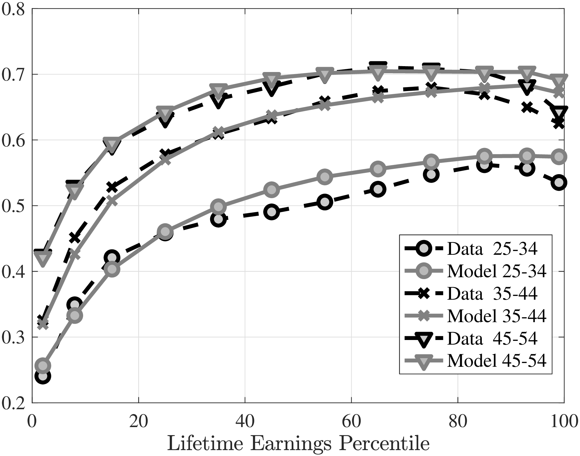
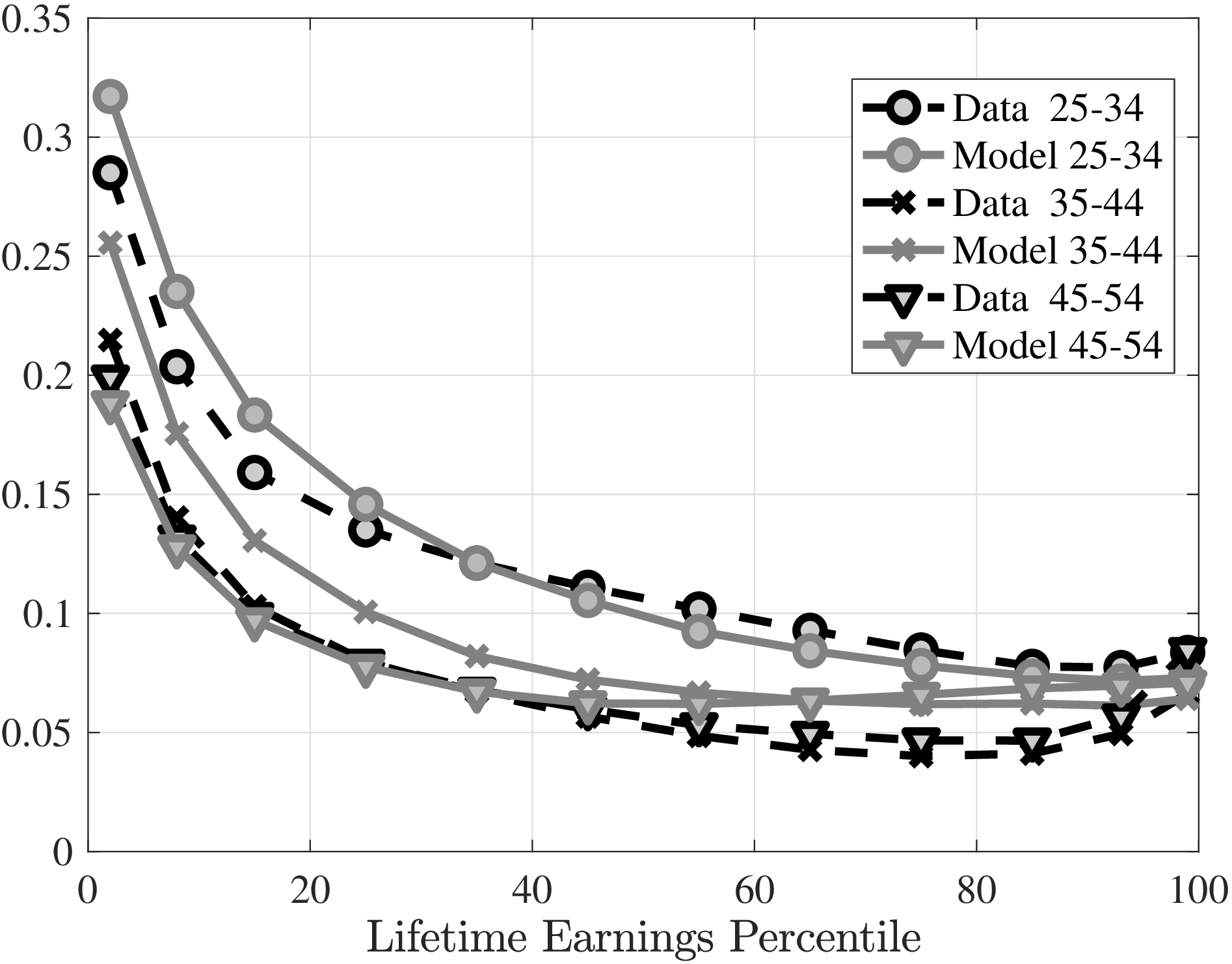
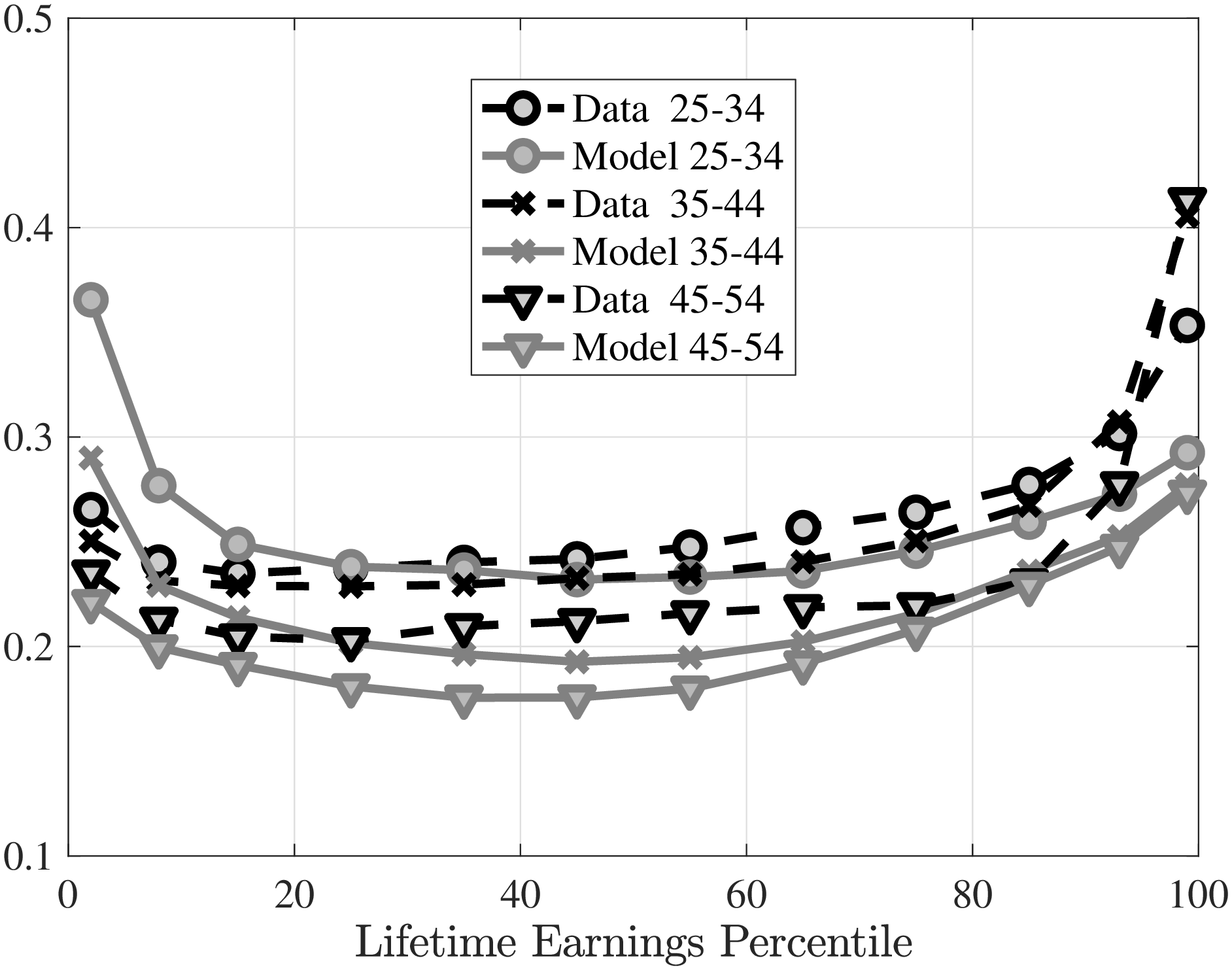
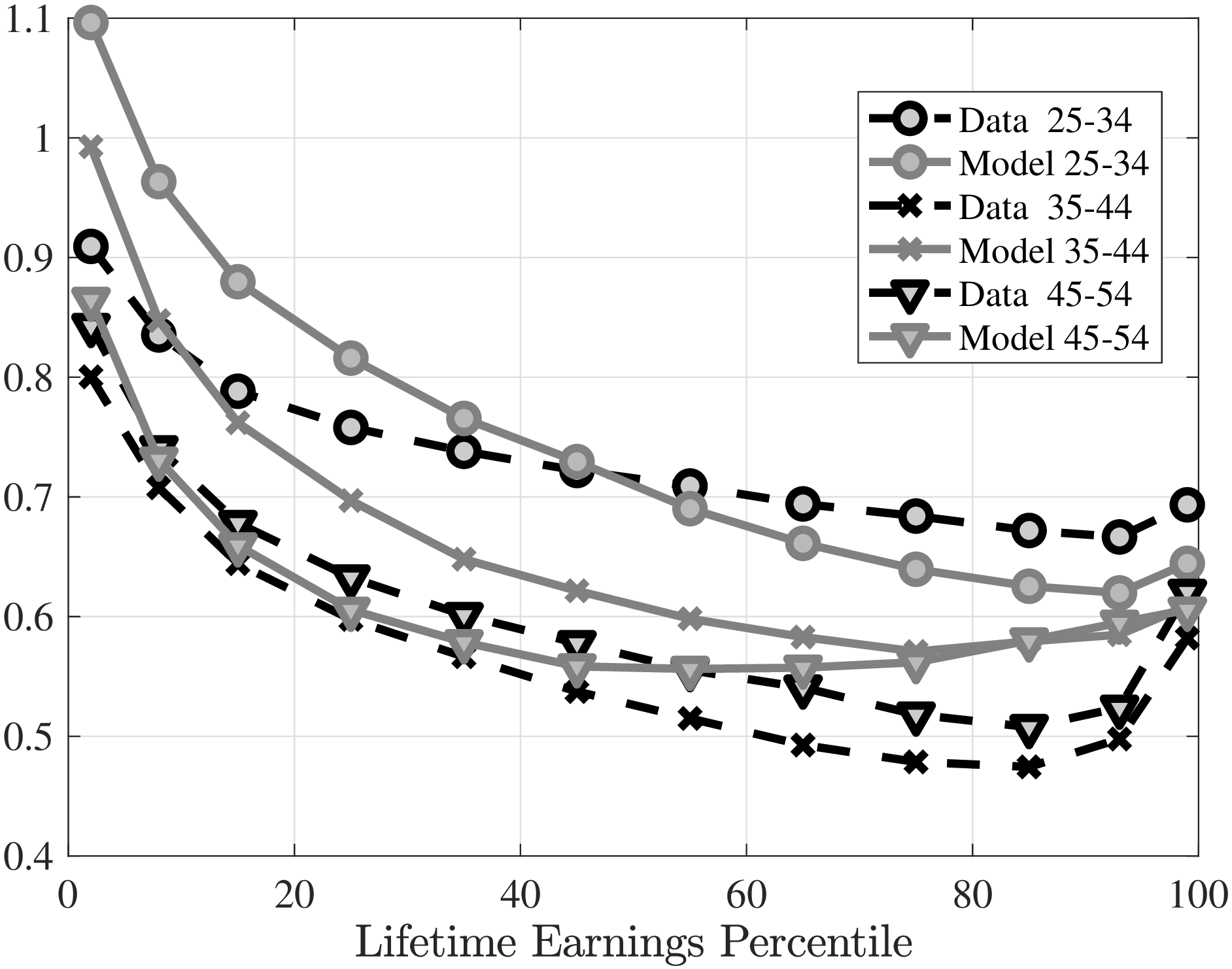
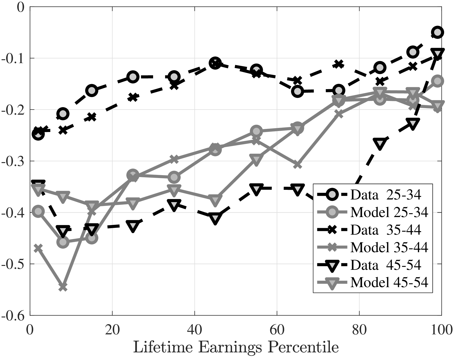
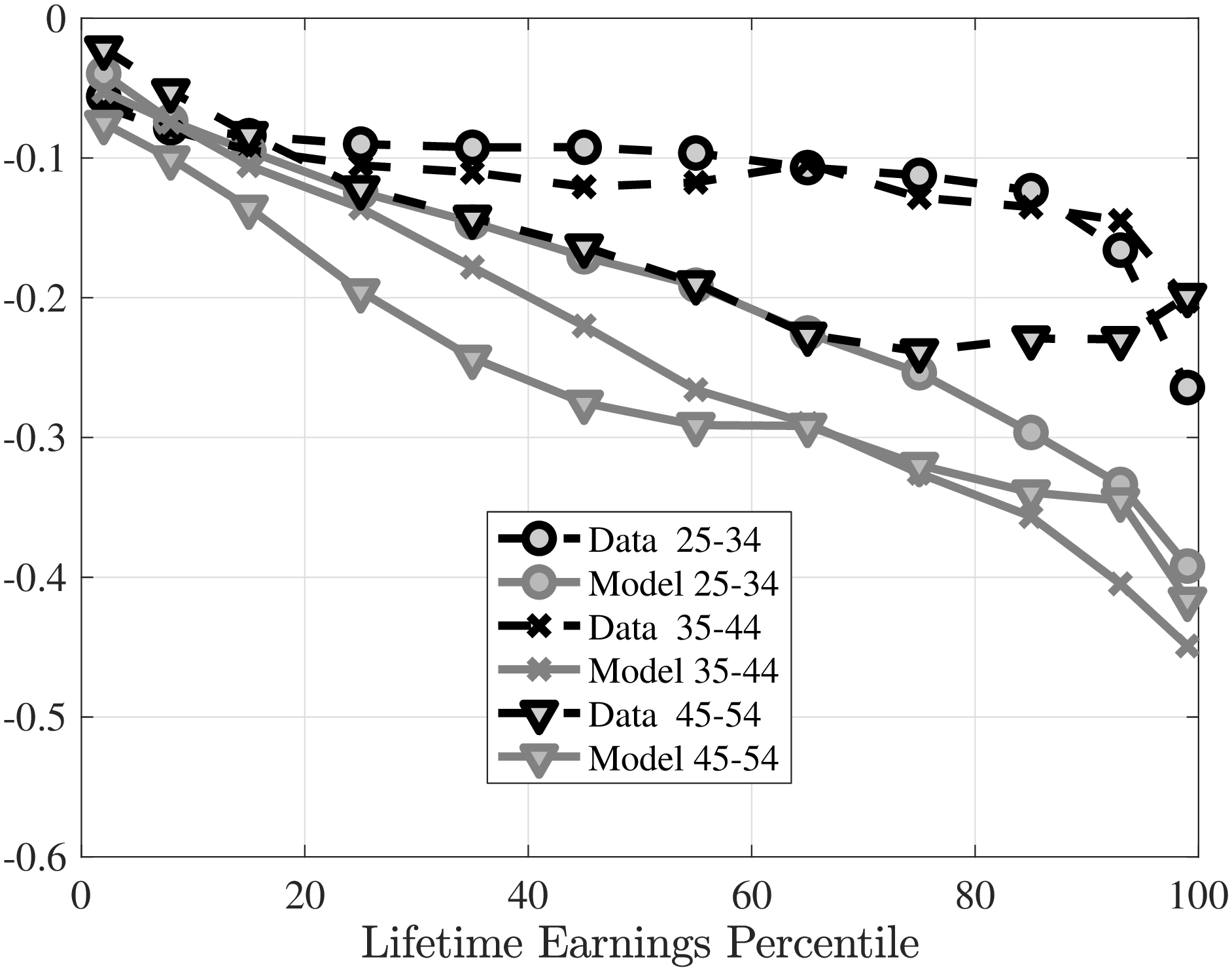
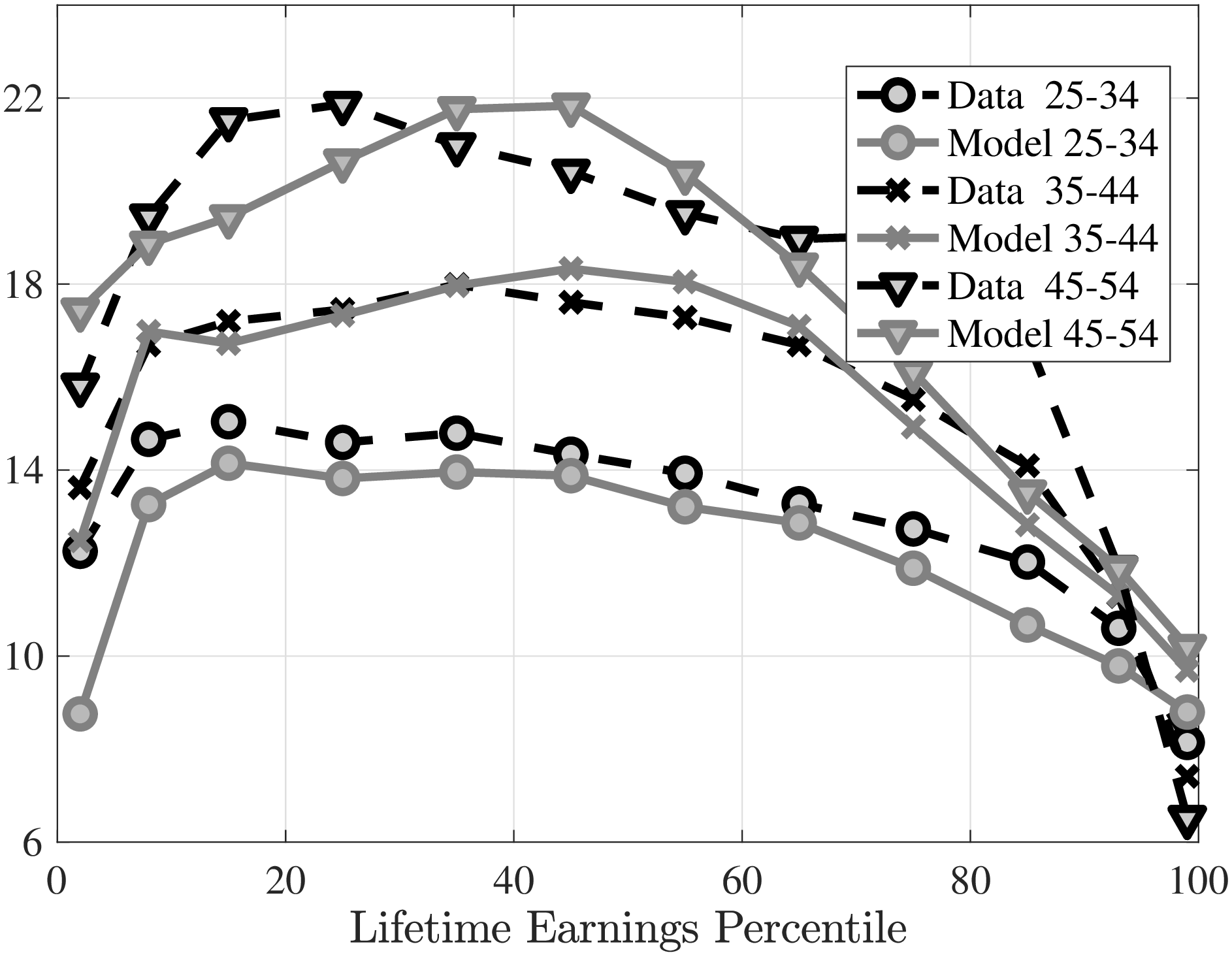
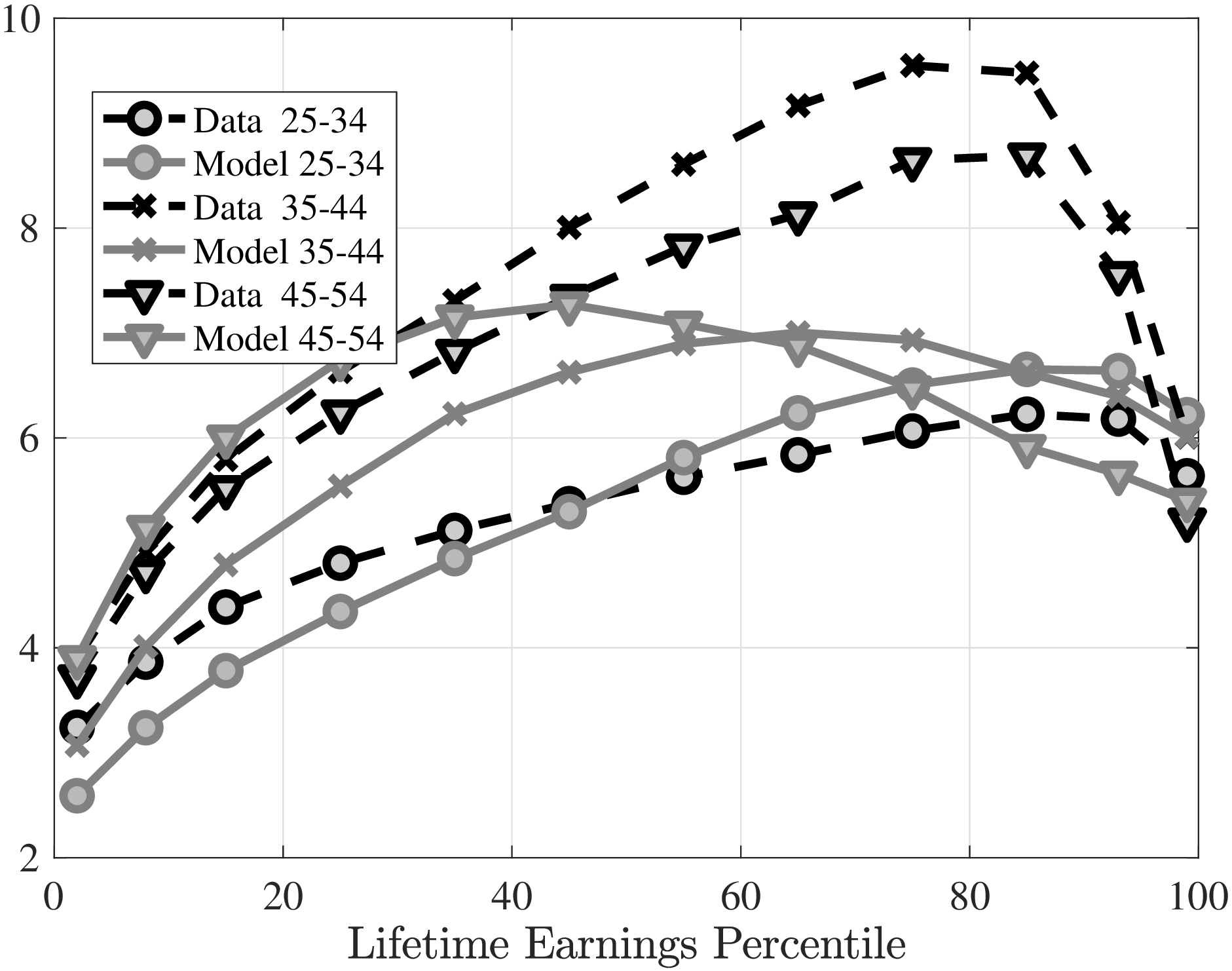
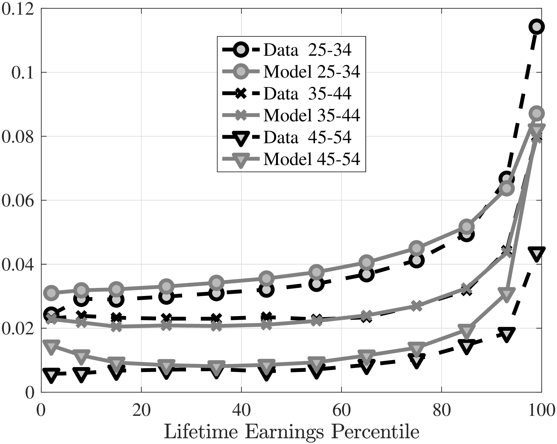
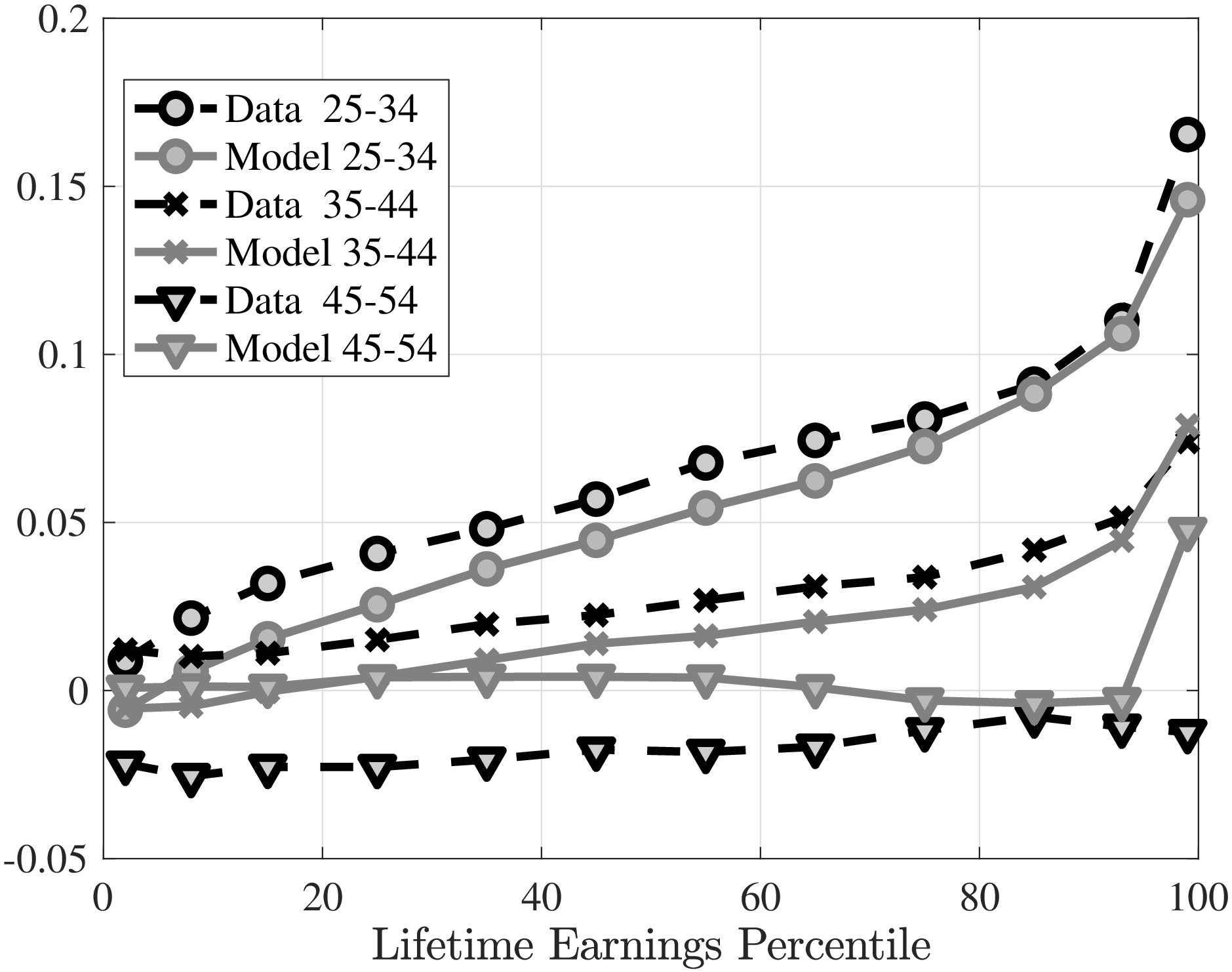
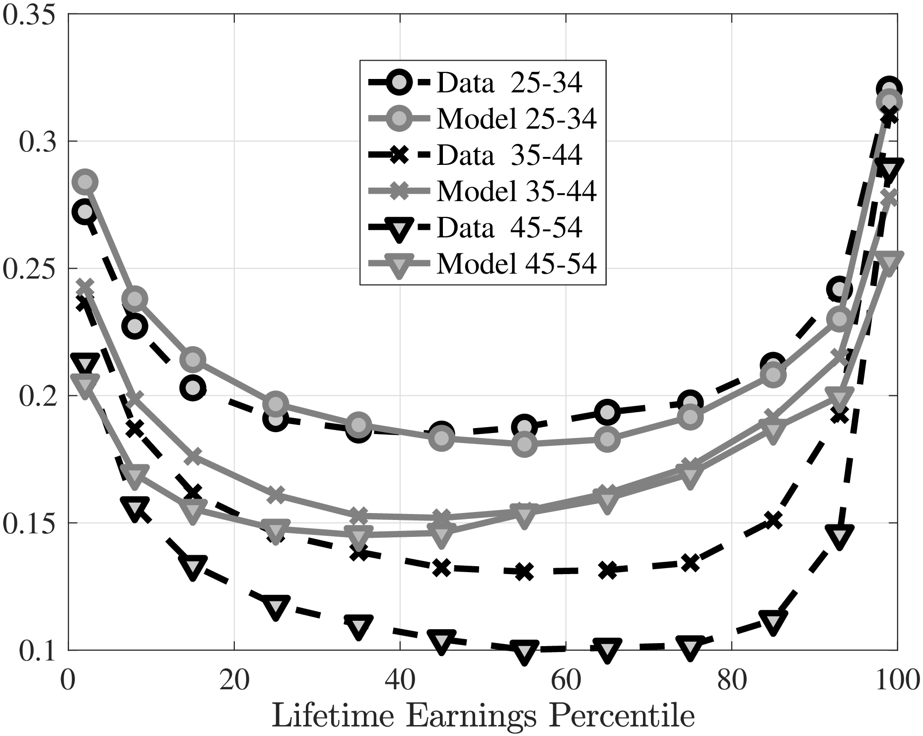
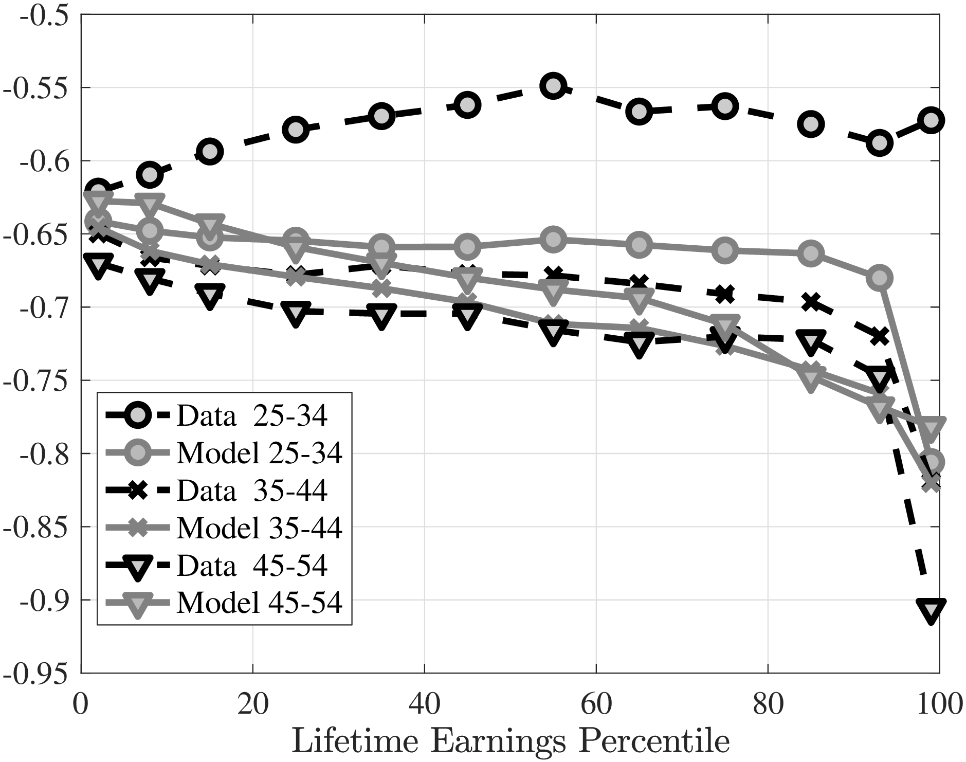
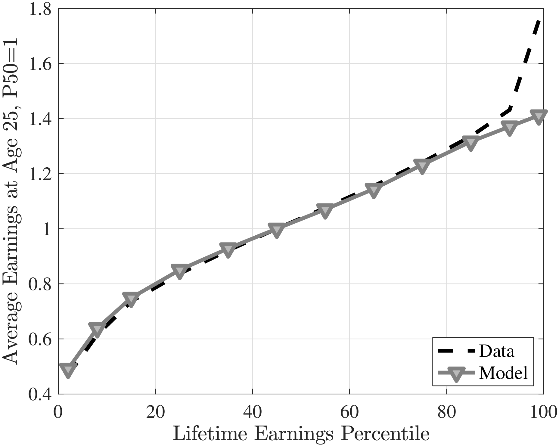
11.2 Parameter Sensitivity
Following Andrews et al. (2017), we compute the sensitivity statistic of our parameter estimates, \(\hat{\theta}\) to moment conditions, \(F(\hat{\theta})\): \[ \Lambda =-\left (G^{\prime}WG\right)^{-1}G^{\prime}W, \] where \(G\)and \(W\) are Jacobian of \(F(\hat{\theta})\) and weighting matrix, respectively.In our model we have 41 parameters and 480 moment conditions, therefore, \(\Lambda\) is a \(41\times 480\) matrix. For brevity, Table D.2 shows the sum of the sensitivity of the shape parameter of Pareto distributed firm productivity, \(\psi _{f}\)to different groups of moments as we defined in Section 4.1—cross-sectional moments of stayer and switcher earnings growth; stayer and E-Switcher probability; average income growth moments for stayers, E-switchers, and U-switchers; and average earnings at age 25. The full matrix is available upon request.
| Cross-sectional | Cross-sectional | Stayer | E-Switch | Stayer | E-Switch | U-Switch | Avg. Earn |
| Stayer | Switcher | Prob. | Prob | Growth | Growth | Growth | at 25 |
| -0.15 | 2.76 | 0.44 | 1.41 | 0.21 | -2.79 | 3.90 | -0.05 |
As we discussed in our identification strategy, this parameter is particularly sensitive to switcher earnings growth moments. Table D.2 confirms our intuition. We show the sensitivity of earnings growth for E- and U- switcher moments over the LE distribution in Figure D.5a. In particular, we average these moments over 3 age groups across the LE distribution for brevity. As we have explained in the paper, dispersion of firm productivity distribution has the most pronounced effect on earnings growth of switchers, and especially those above the median LE. And Figure D.5a confirms this intuition.Notice that higher earnings growth for U-switchers would push up the shape parameter in the Pareto distribution, \(\psi _{f}\), which would imply less dispersion for \(\psi _{f}\). Higher average earnings growth for U-switchers would require smaller scarring effect of unemployment from search capital loss. And the opposite is true for the earnings growth moments for E-switchers. We also confirm that these moments have the most pronounced effect on \(\psi _{f}\) by investigating the sensitivity of other parameters to these sets of moments. These observations are consistent with our informal identification discussion in Section 4.2. Furthermore, while D.2 shows that \(\psi _{f}\) is not very sensitive to average earnings at age 25, this is against our intuition. As we discuss in the paper, initial dispersion of earnings will be most affected by the dispersion of worker productivity, \(\alpha\) but also firm dispersion. Figure D.5a shows that this is indeed the case: Especially, the Pareto firm dispersion parameter has an especially pronounced effect—as expected a negative one—on average earnings at age 25. Interestingly, the effect is slightly positive for workers below the 80th percentile. This is because as we increase \(\psi _{f}\), the dispersion declines but to keep the mean constant at 1, we also shift the location parameter of the Pareto distribution.
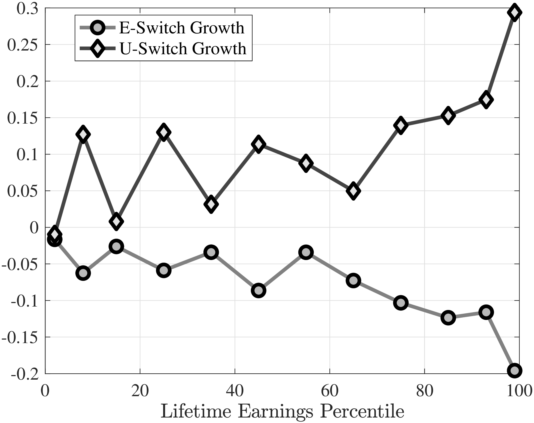
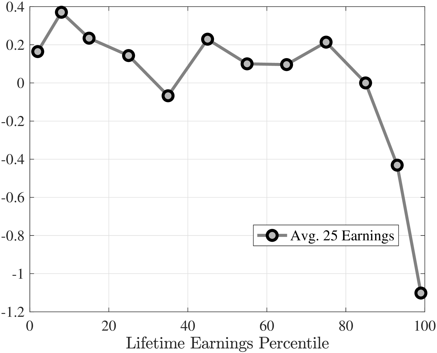
11.3 Additional results
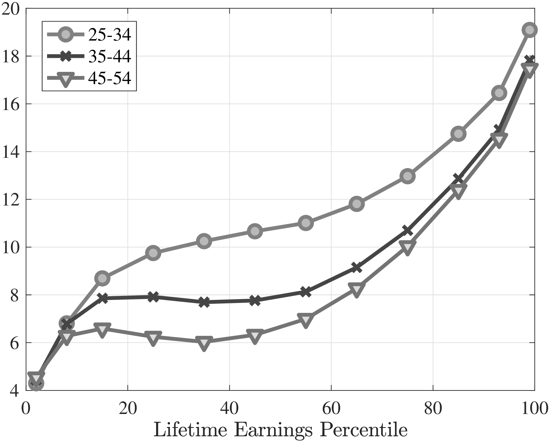
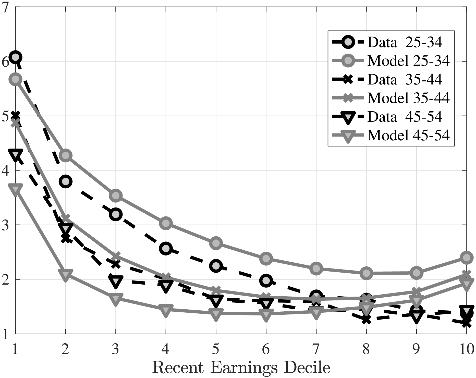
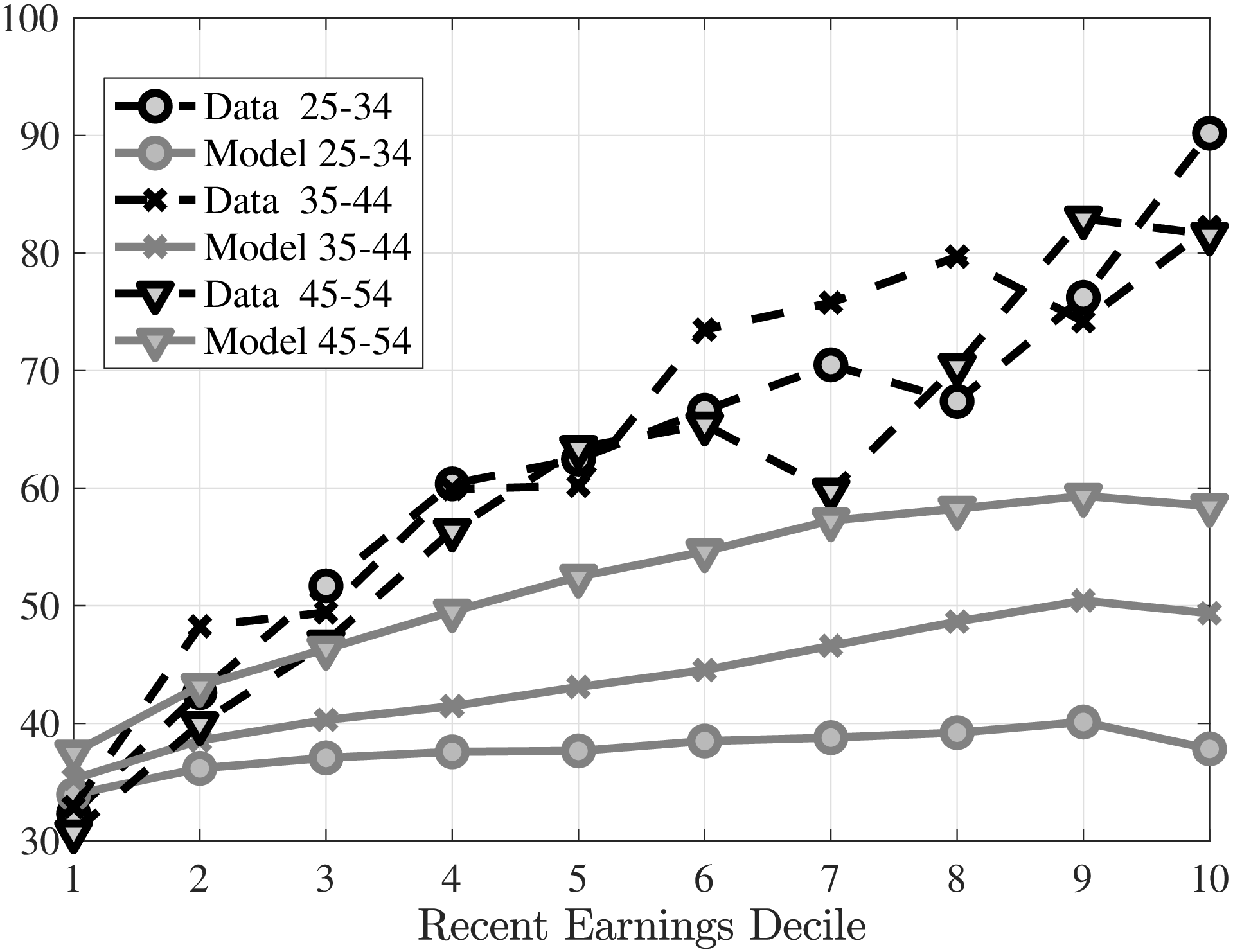
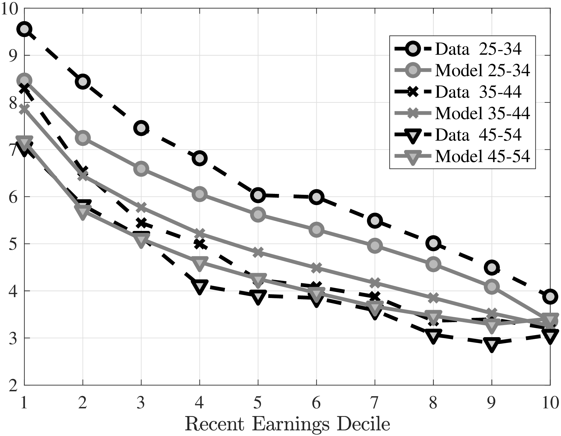
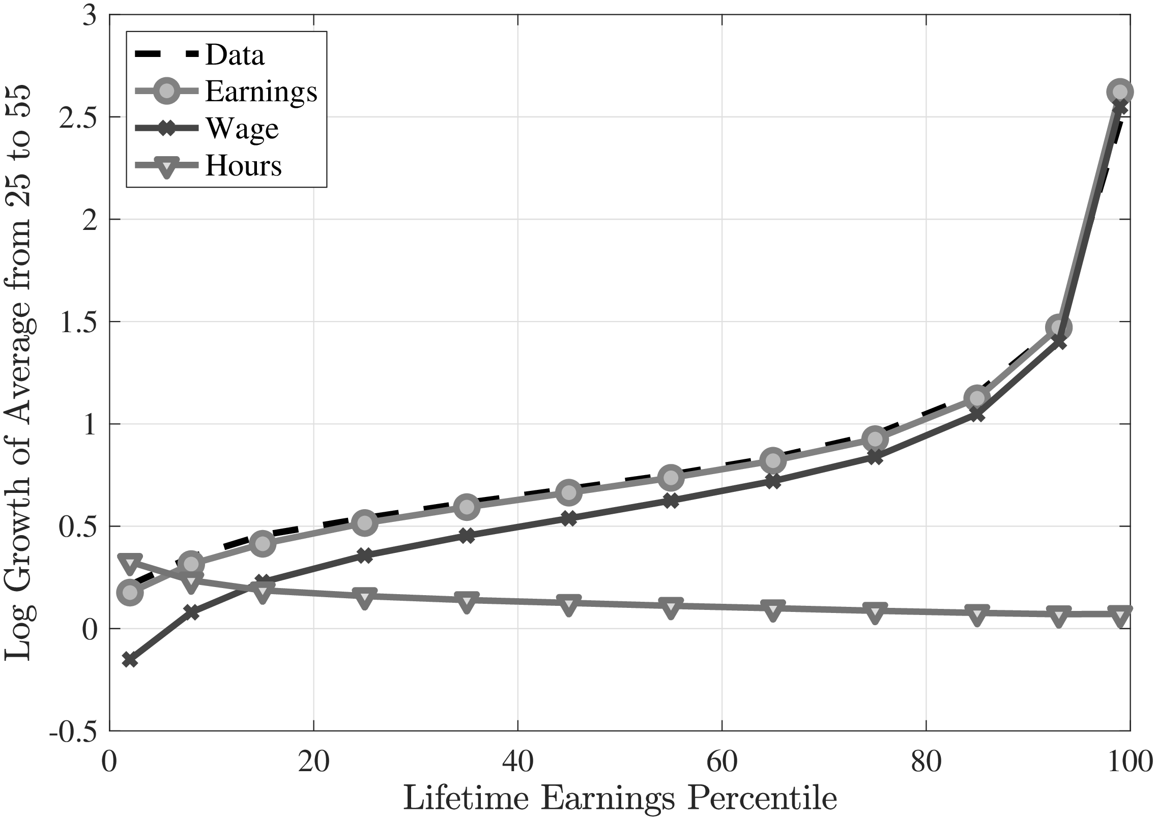
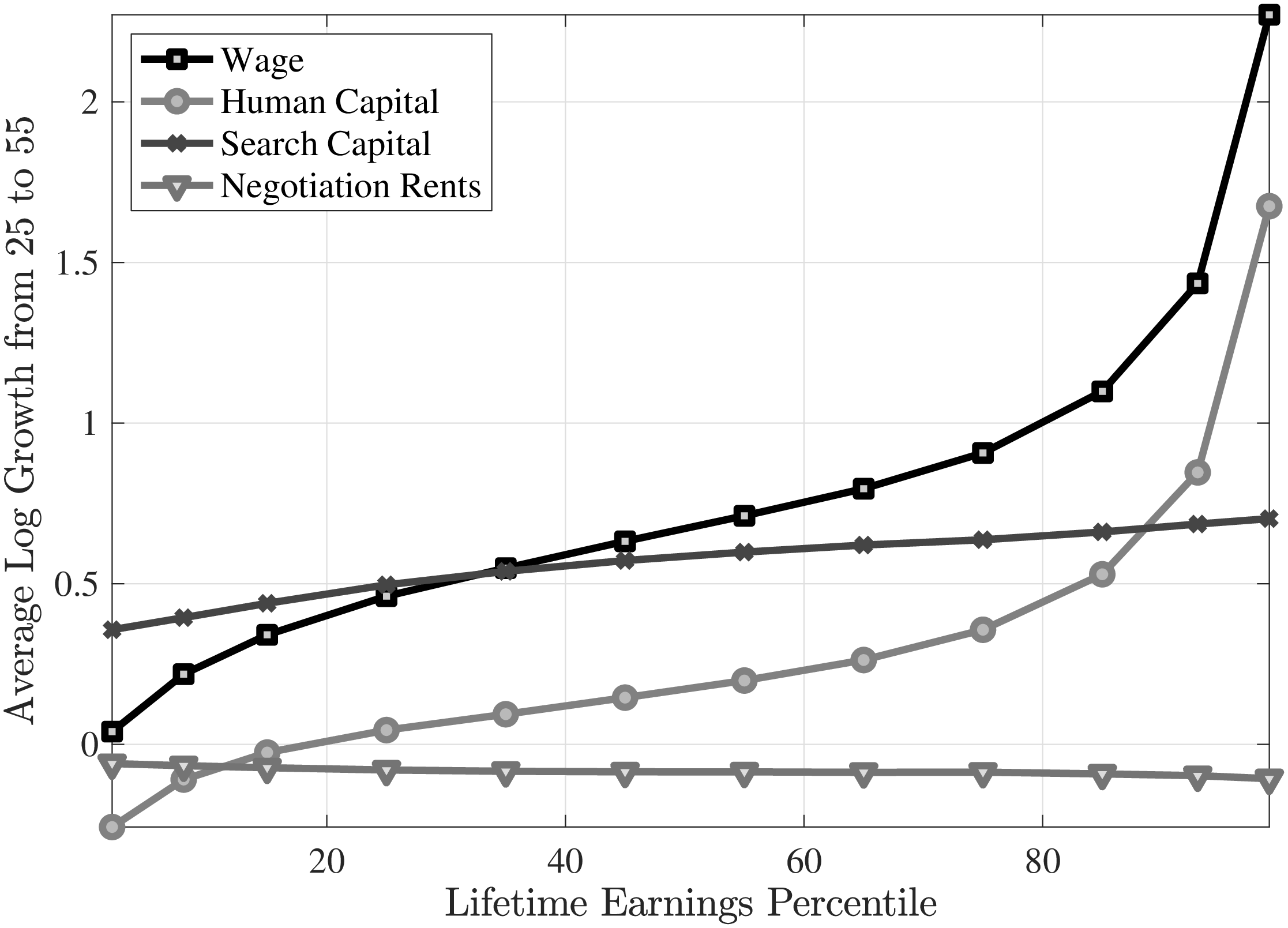
Notes: Notice that the wage growth in the left panel is the log growth of average and in the right panel it is the average log growth of wage. This is because the decomposition in the right panel is only possible when log growth is decomposed.
Footnotes
A long line of literature, dating back to seminal papers by Mincer (1974), Heckman (1976), and Deaton and Paxson (1994), studies the fanning out of inequality over the life cycle. Some explanations of wage growth heterogeneity include human capital accumulation (e.g., Caucutt and Lochner (2020)), learning about workers’ ability (e.g., Jovanovic (1979); Pastorino (2019)), and workers selecting into positions via “tournaments” (Lazear and Rosen (1981)) or according to their comparative advantage (Lise et al. (2016)). See Neal and Rosen (2000) for a comprehensive review of this literature.↩︎
Heterogeneity in lifecycle earnings growth has been well documented in the literature (see, e.g., most recently Guvenen et al. (2021)). However, to the best of our best knowledge, we are the first to decompose lifetime earnings growth differences into job stayer and switcher components.↩︎
Note that a nonemployment spell of at least two full calendar years implies a significantly longer actual spell. Given the duration dependence of job finding rates (Jarosch and Pilossoph 2018), a worker with such a long nonemployment spell is unlikely to have been looking for jobs the entire time.↩︎
Of course, self-employment is an important option in workers’ careers. However, investigating this additional endogenous decision is outside the scope of this paper.↩︎
Clearly, our final sample is highly selective (see Table A.1 for more detail). Appendix A.4 documents the key empirical findings for a broader sample, which are qualitatively similar to our baseline results.↩︎
Career choices are likely based on discounted future earnings. However, there are no market prices for human capital from which we can infer the appropriate discount rate (see Huggett and Kaplan (2016)). We prefer to treat earnings at all ages equally and measure lifetime income in this way (see also Guvenen et al. (2017)). However, we discount future periods in the utility function.↩︎
The results are qualitatively similar for log earnings growth, which excludes earnings below \(Y_{\text{min},t}\).↩︎
Further striking differences exist among top earners. Earnings grow around \(700\%\) for those around the 98th percentile, compared to more than \(5000\%\) in the top 0.2% group (Figure A.5).↩︎
We find similar results when we impose the condition that the main employer accounts for at least 50% of the total income. Results are available upon request.↩︎
The decline in the the fraction of job stayers at the top of the LE distribution can be due to some of the workers leaving the labor force temporarily for schooling (e.g., MBA or law school).↩︎
Guvenen et al. (2021) also investigate how job stayers and switchers across the income distribution differ in earnings growth. However, they document patterns on only higher-order moments of earnings growth (but not on average earnings growth). Thus, we are the first to decompose average earnings growth differentials into job stayer and switcher components.↩︎
Jolivet et al. (2006) show that a sizable portion of direct job-to-job transitions indeed involve wage cuts. Sorkin (2018) argues that some of these differences can be traced to amenity differences across firms. Tanaka et al. (2019) link the earnings declines from direct job switchers to labor force dynamics at both the origin and destination firms.↩︎
For example, if a worker becomes unemployed some time in year \(t\) or \(t+1\), then his earnings in \(t+1\) may reflect earnings from a short-term job in that year. Our approach throughout the paper to dealing with such issues is using the estimated model where we aggregate simulated quarterly earnings to annual, and construct moments in a similar fashion.↩︎
Bowlus and Liu (2013) incorporate endogenous job search in a Ben-Porath human capital model to quantify the relative contributions of each mechanism to life-cycle earnings growth of male high school graduates. They allow for two worker types in job search efficiency and learning ability but assume uniform unemployment risk.↩︎
We have also considered a version with individual-specific \(\zeta\) but not found significant heterogeneity.↩︎
Unemployed workers also lose search capital, negotiation rents and the forgone opportunity of accumulating experience but these fall short of capturing the magnitude of scarring effects of unemployment.↩︎
The option value of recall is higher for workers with higher unemployment risk. Therefore, low LE workers would have accepted lower starting wages when switching to a more productive firm, which would, in turn, imply stronger wage growth on the same job. So, allowing for the value of the recall option in wage bargaining process would be an additional factor why earnings growth of low LE workers is higher for job stayers compared to job switchers and further strengthen our main conclusion that ex-ante heterogeneity in job ladder risk is key for understanding differences in wage dynamics between low and median LE workers.↩︎
Cahuc et al. (2006) argue that this protocol can be micro-founded as the equilibrium of a strategic bargaining game adapted from Rubinstein (1982).↩︎
An alternative is to target percentile-based moments (90-10 differential, Kelley’s skewness, Moors’ kurtosis, etc.), which we have experimented with and found similar results. We target centralized moments as they are less costly to compute and do not overlook valuable information in the tails.↩︎
Following Andrews et al. (2017), we compute the sensitivity, \(\Lambda =-\left (G^{\prime}WG\right)^{-1}G^{\prime}W\), of parameter estimates, \(\hat{\theta}\) to moment conditions, \(F(\hat{\theta})\), where \(G\) and \(W\) are Jacobian of \(F(\hat{\theta})\) and weighting matrix, respectively. This formal sensitivity analysis confirms our informal identification strategy below.↩︎
Some papers have used only worker-side data to identify the firm distribution by relying on the distribution of wages coming out of unemployment (e.g., Lise (2013)). This approach is not reliable in an environment with worker heterogeneity as shown in Barlevy (2008).↩︎
In our simulations, less than 0.2% of direct job-to-job switches lead to a wage cut larger than 25%.↩︎
Polachek et al. (2015) also estimate a fat tailed distribution of learning ability in a human capital production function. Gabaix et al. (2016) argue that the “high-growth” worker types, as opposed to a random growth mechanism, are key for explaining the rising top income inequality.↩︎
We have experimented with log-normally distributed firm productivity and found that a Pareto fits the data better. Hubmer (2018) uses a different search model and reaches a similar conclusion.↩︎
We experimented with AR(1) productivity shocks and found the persistence to be low around 0.5. We have also considered alternative distributions for innovations such as those exhibiting skewness and did not find significant improvement in the objective value.↩︎
The weighting matrix, \(W\), assigns a 15% weight to the first two sets of moments (i.e., cross-sectional moments of job stayers and switchers), a 30% weight to the third and fourth sets (i.e., the fraction of job stayers, EE—switchers, and EUE—switchers and their average wage growth), and a 10% weight to the moments on average earnings at age 25 for each LE group. We chose not to use the optimal weighting matrix because efficiency is not a concern, as our moments are precisely estimated thanks to the sheer sample size. This also applies to Altonji and Segal (1996)’s identity matrix, which is about minimizing small sample bias. We have yet experimented with equal weighting matrix and come to roughly similar conclusions (available upon request).↩︎
Note that the interquartile range of \(\beta\) also increases from less then 0.005 at the bottom to more than 0.03 at the top, which is a direct feature of the fat tail of the Pareto distribution. The standard deviation of \(\beta\) in the population is estimated to be 0.017, in line with the estimates in the literature using different methodologies and datasets (Huggett et al. (2011) and Guvenen et al. (2021)).↩︎
We would like to remind that the old (\(o\)) and young (\(y\)) ages in the model do not correspond to the calendar age in our simulations. Due to the stochastic aging process, there are old (\(o\)) workers in the model, even at earlier ages in the simulation.↩︎
Jarosch (2015) develops a two-dimensional job ladder model with jobs also differing in unemployment risk and uses the life-cycle variation in unemployment risk to estimate this model.↩︎
Though these differences are significant, they are not as large as job loss heterogeneity. Cairo and Cajner (2017) also show that more educated workers have similar job finding rates but much lower and less volatile separation rates than their less educated peers.↩︎
Recall that job finding rate has a pronounced effect on the average earnings loss of U–switchers. The model can successfully capture its variation along the LE distribution (Figure 8d), with slightly smaller losses for high LE workers than in the data. Thus, if their job finding rate were higher, we would have seen even smaller earnings losses for high LE U–switchers. The failure to capture their higher job finding rates, however, is not very consequential for our main results because they are much less likely to be unemployed to begin with.↩︎
Interestingly, in contrast to the literature that estimates a much smaller offer arrival rate for employed workers than for the unemployed (e.g. Jarosch (2015), Schaal (2017)), our estimates for \(\lambda _{0}\) and \(\lambda _{1}\) are comparable in level, which has implications for unemployment insurance. For example, a high level of \(\lambda _{1}\) increases the value of work, and reduces moral hazard, thereby increasing the optimal replacement rate (Chetty (2008)).↩︎
Using Danish data, Bagger et al. (2014) and Lentz et al. (2018) estimate contact rates to be increasing in worker type too.↩︎
We decompose lifetime earnings growth into wage and hours growth components (Figure D.8a). Earnings growth is less dispersed than wage growth between LE groups, especially in the bottom half of the LE distribution, due to higher lifetime employment growth of bottom LE workers.↩︎
Recall that the model cannot capture higher job finding rates for higher LE workers seen in the data (Figure 6d). Even though differences in \(\lambda _{0}(\alpha)\) is less important compared to \(\delta (\alpha)\) for our results, larger variation in \(\lambda _{0}(\alpha)\) would have surely generated stronger role for heterogeneity in job ladder risk in the bottom half of the LE distribution.↩︎
The growth in search capital is measured as the log change in firm productivity \(\mathbb{E}\left [p_{j(i,55)}-p_{j(i,25)}\right]\), and the growth in negotiation rents is measured as the change in the log piece rate \(\mathbb{E}\left [r_{i,55}-r_{i,25}\right]\).↩︎
As we previously discussed, to maintain tractability for the model we assume the value of recall option is not considered in the wage bargaining process. If we had allowed for it, it would have contributed to wage growth differences through the piece rate. However, as we show here the contribution of the negotiation capital over the life cycle is small relative to human capital and search capital components. So, the role of recall option in wage bargaining process would be quantitatively small.↩︎
St. Louis Fed and University of Toronto; serdar.ozkan@utoronto.ca; www.serdarozkan.me Jae Song 2 2 Social Security Administration; jae.song@ssa.gov Fatih Karahan 3 3 Amazon; yfkarahan@gmail.com; sites.google.com/site/yfatihkarahan/↩︎
We cannot rank people by their lifetime earnings, since in the SIPP we don’t observe the entire earnings history of individuals. Therefore, we condition workers by their average past wages.↩︎