Dissecting Idiosyncratic Earnings Risk

Elin Halvorsen; Hans A. Holter; Serdar Ozkan; Kjetil Storesletten

Abstract

This paper examines whether nonlinear and non-Gaussian features of earnings dynamics are caused by hours or hourly wages. Our findings from the Norwegian administrative and survey data are as follows: (i) Nonlinear mean reversion in earnings is driven by the dynamics of hours worked rather than wages since wage dynamics are close to linear, while hours dynamics are nonlinear—negative changes to hours are transitory, while positive changes are persistent. (ii) Large earnings changes are driven equally by hours and wages, whereas small changes are associated mainly with wage shocks. (iii) Both wages and hours contribute to negative skewness and high kurtosis for earnings changes, although hour-wage interactions are quantitatively more important. (iv) When considering household earnings and disposable household income, the deviations from normality are mitigated relative to individual labor earnings: changes in disposable household income are approximately symmetric and less leptokurtic.

JEL Codes: E24, H24, J24, J31. Keywords: Earnings dynamics, Income shocks, Insurance, Wages, Hours, Higher-order earnings risk, Skewness, Kurtosis, Machine learning.

1 Introduction

The nature of income dynamics and the distribution of idiosyncratic shocks are crucial for behavioral choices of consumption, savings, and leisure, and influence the design of optimal social insurance and taxation. While the early literature studying idiosyncratic income fluctuations focused mostly on linear and symmetric models of risk, recent contributions have explored nonlinearities and nonnormalities (e.g., Arellano et al. (2017); Guvenen et al. (2014); Guvenen et al. (2019)). In particular, this literature has documented that the persistence of innovations is not uniform but exhibits systematic asymmetries—for example, that large negative earnings shocks are less persistent than positive changes—and that the distribution of innovations to income displays strong left skewness and excess kurtosis relative to normally distributed shocks. Much of this literature has focused on fluctuations in individual annual earnings. However, many questions in economics, such as optimal taxation and consumption-savings choices, require that one studies the dynamics of disposable household income rather than individual labor earnings before taxes. Moreover, it is important to also understand the dynamics of each of the components that labor income comprises: hours worked and hourly wages.¹

This paper decomposes earnings shocks into changes in hours and changes in wage rates and studies the extent to which the nonlinear and non-Gaussian aspects of male earnings dynamics are driven by hours, wages, or their interactions. ² We also examine the role of specific sources of large earnings shocks such as job changes. Finally, we examine the extent to which the non-Gaussian aspects of male earnings changes are passed through to household earnings and household disposable income. We study these questions using nonparametric methods building on Guvenen et al. (2014); Guvenen et al. (2019), which enables us to detect the sources behind the nonnormalities and nonlinearities in a descriptive and intuitive way. To this end, we use panel data from a combination of administrative registers (e.g., annual tax records and employment registers), covering the entire population in Norway. Furthermore, we link the Norwegian Labor Force Survey (AKU) data set to these administrative records to derive a high-quality measure of hours worked. Specifically, we employ machine learning techniques to estimate a model for the actual annual hours in the AKU as a function of observables available in the registry data. We then apply this model to the entire workforce to impute a similar labor hours measure. This imputation procedure is an independent contribution of our paper.

We start by decomposing earnings growth into hours and (hourly) wage components conditional on workers’ age and past earnings. For workers in the middle of the earnings distribution, hours and wage growth are about equally important in accounting for large changes in earnings, whereas small earnings changes are mainly driven by wage growth. Low and high earners exhibit different patterns, however. For individuals with low past earnings, hours changes account for a larger fraction of earnings growth than does wage growth. For high earners, this pattern is reversed, with wage growth accounting for most of their earnings fluctuations. The main events associated with large negative or positive earnings shocks are transitions in and out of long-term sickness, transitions between full-time and part-time work, and job changes.

We next document that the persistence of earnings changes in Norway is highly asymmetric, a finding broadly consistent with other studies for U.S. and Norwegian workers (c.f., Arellano et al. (2017); Guvenen et al. (2019)). Small shocks and large increases are essentially permanent, whereas large declines are transitory for most workers. The exception is the high earners, for whom negative changes are highly persistent and positive ones are more transitory. Exploiting the administrative nature of our data—which includes even those who drop out of the workforce—our methodology allows us to study effects working through both the intensive and the extensive margins of labor supply.

We investigate the dynamics and mean reversion patterns of hours worked versus hourly wages in order to understand the drivers of the nonlinear persistence of earnings. We uncover a sharp dichotomy between hours and wages. Changes in wage rates are highly persistent. This holds true for both positive and negative changes, and for small and large changes alike. In contrast, the persistence of changes in hours worked turns out to be highly nonlinear: moderate and large reductions in hours worked tend to be transitory and have mostly disappeared five years after an initial fall, whereas increases in hours worked are permanent. This holds true for all workers except for those with the highest recent earnings. We conclude that the nonlinear persistence of individual earnings changes in Norway is mainly driven by hours worked and not hourly wages. Namely, large earnings declines for the majority of workers are transitory because they are, to a larger extent, driven by hours declines, which are transitory. Again, the exception is the high earners, for whom declines have a somewhat larger persistence because earnings reductions for these workers are primarily driven by wage declines, which are persistent.

We then turn to the distribution of individual earnings changes in Norway. A first observation is that its higher-order moments and their variation over the life cycle and between income groups are qualitatively remarkably similar to those reported for U.S. workers (see Guvenen et al. (2019)). In both countries, the variance of earnings growth declines in age and in recent earnings, although the volatility is larger in the U.S. than in Norway. Earnings growth is not symmetric but negatively skewed, and the left skewness becomes more pronounced as individuals get older or their earnings increase. Moreover, this distribution is highly leptokurtic and even more so for the high-income or older worker. We conclude that, despite the differences between Norway and the U.S. in their welfare state and labor market institutions, the nonnormalities and nonlinearities in earnings dynamics are very similar, which might reflect similar underlying economic mechanisms (see Karahan et al. (2019); Hubmer (2018)).

We study the distributions of hours and wage growth and their role in driving the higher-order moments of earnings growth and find that both hours growth and wage growth display non-Gaussian features. Both are left skewed, albeit less so than earnings growth. Moreover, both display excess kurtosis, with hours growth having higher kurtosis than earnings growth. To quantify the importance of hours and wage growth in the higher-order moments of earnings growth, we apply an exact statistical decomposition where the skewness (kurtosis) of log earnings growth is a weighted sum of the skewness (kurtosis) of log hours and wage growth plus a residual co-skewness (co-kurtosis) term that broadly captures whether large hours and wage changes coincide. All terms contribute to the negative skewness of earnings growth, with co-skewness being the main component (i.e., workers experience large declines in hours and wages simultaneously). Similarly, the co-kurtosis term is the largest contributor to the excess kurtosis.

We also investigate the role of job changes—one of the main events associated with large earnings changes—in driving the skewness and kurtosis of earnings changes. We find that the distribution of earnings growth for job switchers exhibits weaker negative skewness and less excess kurtosis compared to the distribution for job stayers. Furthermore, there are very few job switchers relative to the number of job stayers. Therefore, the skewness and kurtosis of earnings growth tend to be driven by job stayers.

Finally, we examine how the dynamics of household earnings and disposable income differ from male earnings dynamics. Disposable income is substantially less volatile than male earnings because of spousal and public insurance. Relatedly, growth in household earnings and disposable income is less negatively skewed, with disposable income growth being approximately symmetrically distributed. Thus, we conclude that the Norwegian system of taxes and transfers provides substantial insurance against tail risk in income.

Our paper is structured as follows. We review some of the related literature on earnings dynamics in Section 2. Section 3 describes the data and empirical methodology. In Section 4, we decompose earnings risk into changes in hours and changes in wage rates and study their dynamics and contributions to earnings growth. Section 5 studies the higher-order moments of wage and hours growth and their contributions to the higher-order moments of earnings growth. It also examines how the higher-order moments are affected when going from male labor earnings to household earnings and household disposable income. We finally conclude in Section 6.

2 Related Literature

A number of empirical studies have focused on the distributional properties of income shocks, including classic contributions by Lillard and Willis (1978), Lillard and Weiss (1979), MaCurdy (1982), and Abowd and Card (1989). Most of this work has been based on survey data on individual labor earnings. Because of limited sample sizes, the approaches in these studies have been parametric. Guvenen et al. (2014); Guvenen et al. (2018) rely instead on administrative data from the U.S. Social Security Administration (SSA) to study the distribution of individual annual earnings changes. They document that male earnings changes are strongly negatively skewed (negative shocks have a thicker tail than positive shocks) and more leptokurtic than a normal distribution (both positive and negative shocks have thicker tails). However, several important questions cannot be answered because of SSA data limitations. One shortcoming is the lack of detailed information on components of annual individual earnings, such as hours worked, hourly wages, unemployment spells, and other nonworking spells. Another shortcoming is missing information on other household members and other types of income such as government taxes and transfers and capital income. The Norwegian data used in this paper contain all this information and are the basis of our investigation.

Some recent papers consider higher-order moments of household labor income risk and household disposable income risk but focus mainly on the variation over the business cycle. Pruitt and Turner (2018) use Internal Revenue Service (IRS) data to study the distribution of household labor income risk over the business cycle. In line with our findings for Norway, they find that household labor income growth in the U.S. is significantly less negatively skewed than individual earnings growth. Busch et al. (2018) use data from the U.S., Germany, and Sweden to study variations in higher-order earnings risk over the business cycle. They argue that the family and the welfare state are only moderately efficient in terms of mitigating business cycle risk.

In a contemporaneous paper, De Nardi et al. (2021) also study the higher-order moments of household income before and after taxes and transfers as well as the higher-order moments of hours and wage growth using administrative data from the Netherlands. In line with our findings for Norway, they find that wage growth is negatively skewed and that there is significant insurance from the family and the welfare state. Like us they also find that hours growth is relatively more important for explaining the earnings growth of low earners compared to high earners. However, unlike our paper, they do not study the asymmetric mean reversion of earnings. Furthermore, De Nardi et al. (2021) rely on an employer-reported hours measure in the Dutch register data, which does not include overtime for full-time workers.³ We instead impute a measure of actual hours worked based on the Norwegian Labor Force Survey, combined with detailed government administrative records, one of which is employer-reported contracted hours. We document below that this contracted hours measure contains large and systematic measurement error (henceforth m.e.) relative to survey data on actual hours in the Norwegian context.

While our paper and the papers discussed above pursue a nonparametric approach to studying income shocks, Arellano et al. (2017) put more structure on the income process. They develop a quantile-based panel data framework to study the nature of income persistence and the transmission of income shocks to consumption where log earnings is modeled as the sum of a general Markovian persistent component and a transitory innovation. Using both the Panel Study of Income Dynamics (PSID) and Norwegian register data, they document that the persistence of earnings shocks is nonlinear (asymmetric). Our results for earnings are in line with their paper, and our contribution is to extend the study of nonlinearities to hours and wage rates.

Our paper also contributes to the broader literature on idiosyncratic risk and risk sharing, which includes Cutler and Katz (1992), Deaton and Paxson (1994), Attanasio and Davis (1996), Blundell and Preston (1998), Krueger and Perri (2005), Blundell et al. (2008), and Heathcote et al. (2014). Blundell et al. (2014) study insurance in Norway through from the welfare state and the family. They find that the welfare state provides a large reduction in the variance of persistent and transitory shocks relative to individual labor income and more so for low- and medium-skilled workers relative to high-skilled workers. Our findings are in line with these results.

3 Data and Methodology

In this section, we describe our data sources and the machine learning algorithm we employ to impute actual work hours in the register data. We also lay out the empirical methodology for studying earnings, hours, and wage changes.

3.1 Data Sources on Income and Labor Supply

Our analysis uses data from four different data sources between 1993 and 2014. The first data set is Administrative Tax and Income Records, which contains a set of detailed information on income and taxes for the entire Norwegian population from 1993 onward. In addition, this register contains information on age, gender, household composition, country of origin, and education. Our measure of labor earnings is comprehensive and includes wages and salaries from all employment, including bonuses and other irregular payments. We exclude income from self-employment and also exclude individuals with significant self-employment income from the sample, mainly because we do not have data on labor supply for self-employed individuals.⁴

Tax records are of high quality because most information is third-party reported to the tax authorities, and very little is self-reported. Employers, banks, brokers, insurance companies, and any other financial intermediaries are obliged to report information on earnings payments, the value of assets owned by the individual and administered by the financial intermediary or employer, as well as information on the income earned on these assets. Capital income is measured as the sum of positive interest, dividends, and realized capital gains and losses but without deductions for interest expenses. Moreover, the tax records contain information on transfers and income taxes. Transfers include unemployment benefits, sickness benefits, paid parental leave, remuneration for participation in various government activity programs, disability benefits, public pensions, and other social welfare payments.

For most of our analysis, the basic tax unit is an individual. For our household-level analysis, we use family identifiers from the population register, pooling the individual incomes of spouses for both married and cohabiting couples to calculate household income. Household income is equivalized using the OECD equivalence scale. All values are deflated using the (Laspeyres) Consumer Price Index.

The second data set is maintained by the Norwegian Social Security Administration and contains the start and end dates of spells for unemployment, parental leave, sickness, and disability benefits at the daily level. We use this information in our impution model.

The third data set we use is the Employment Register, which is a matched employer-employee data set of the universe of employers and employees in Norway. All employers are required to report contractual hours, employment duration, sector, and industry to the government. Information about contractual hours of work is limited to the period from 2003 to 2014, since prior to 2003 only full-time and part-time hours was reported.⁵ The Employment Register covers the entire labor force, except for self-employed workers and freelancers. This amounts to 90% of the labor force and 77% of the prime-age population (25 to 60 years old). For individuals with multiple jobs during the year, we define main employment as the job that accounts for the largest share of annual earnings and measure annual “register hours” as the sum of contractual hours worked in all jobs.

Finally, to measure actual annual hours worked for the entire population, we use data from the Norwegian Labor Force Survey (AKU) in combination with register data. The next section lays out our measurement and imputation procedure and motivates why our approach provides a better measure of labor supply than the register hours.

3.2 Measuring and Imputing Actual Hours of Work

3.2.1 Measuring Annual Hours Worked in the AKU

The AKU is the basis of official Norwegian employment statistics, comparable to the Current Population Survey (CPS) for the U.S. It is a representative survey of all residents ages 15-74, covering 24,000 people each quarter. The sample is a rotating panel where each participant is interviewed for eight consecutive quarters. We focus on 2003-2014 and restrict the sample to individuals ages 25-60. We impute annual hours for individuals for whom we have at least three quarterly observations in a calendar year. This yields a final sample of 35,909 men and 35,175 women.

Survey participants report two measures of labor supply during the week preceding the interview: actual hours worked last week and regular (contracted) hours last week. By relying on remembering very recent events, the AKU measures of hours worked are robust to standard recall bias. The survey week is randomly drawn within the quarter.⁶ See Appendix A.3 for a more comprehensive description of the Labor Force Survey.

Given reported labor supply for four weeks in a year, we impute the total annual hours in year $t$ as $h_{t,j}^{LFS}=13\cdot \sum _{q=1}^{4}h_{t,q}^{LFS}$, where $h_{t,d}^{LFS}$ is weekly hours in quarter $q$ of year $t$ and $j$ represents either actual hours or contracted hours.⁷

The next subsection motivates why we use the actual hours variable in the AKU as our main measure of labor supply instead of the contractual hours measure in the administrative data. We also estimate m.e. for the contractual hours measure in the Employment Register using a similar variable from the AKU.

3.2.2 Actual Hours versus Register Hours

The measure of contractual hours in the Employment Register has significant weaknesses as a measure of actual hours worked, and we believe that the AKU actual hours variable offers a better measure of actual labor supply for four reasons. First, Statistics Norway uses this survey to calculate official statistics on aggregate employment and unemployment (instead of contractual hours information in the employment register). Therefore, it is conducted using modern survey techniques, designed to minimize m.e. and to provide a precise measure of actual hours worked.

Second, “contractual hours” measures the regular hours in the employment contact. This measure of labor supply is conceptually different from actual annual hours worked, which is what we need for our purposes. In particular, contractual hours do not include overtime because the Employment Register was originally administered by the Social Security Administration to calculate work-related benefits, which does not cover overtime. Moreover, the register does not cover employment that amounts to less than four hours per week or seven days per job spell.

Third, even as a measure of regular hours, contractual hours in Norwegian register data contain substantial m.e. because employers often fail to update changes in employment spells or contractual hours. While earnings and employment matter for taxes and transfers from the Norwegian government, neither hours worked nor contractual hours play any role for taxes and transfers. The Employment Register does, therefore, not have an incentive to enforce accurate reporting of contractual hours and misreporting does not have any repercussions for the employer.⁸ This m.e. can be quantified using the AKU measure of contractual hours. We interpret the variable contracted hours in the AKU survey as the respondents’ perception of register hours in the Employment Register. Moreover, all individuals surveyed in AKU can be matched to the register data. The availability of two independent measures of contractual hours—self-reported and reported by the employer, respectively—allows us to estimate the magnitude of the m.e. for contractual hours in the register data. Assume that m.e. in growth in (the log of) contracted hours in both AKU and register data is classical (i.i.d.). Then the variance of this m.e. can be estimated as the difference between the variance of log hours growth in the register data and the covariance between contracted log hours growth in AKU and the register data. This estimation procedure implies a variance of classical m.e. of 0.061 and 0.047 for young and old men, respectively. Thus, m.e. accounts for 65% and 83% of the variance of contracted hours growth for young and old men, respectively. For comparison, this is the same order of magnitude of m.e. that Heathcote et al. (2014) estimate for male hours growth in the PSID.⁹ We interpret this finding as an indication that contractual hours in AKU exhibit substantial m.e., of a magnitude comparable to that of the PSID.

The fourth and most important reason for actual hours being a better measure than register hours is that observed earnings changes have a much stronger correlation with actual hours changes than with register hours changes. To show this, we rank individuals present in the Labor Force Survey into 10 bins based on their one-year earnings changes, where earnings data are from the register data. For each bin, we plot the log change of average earnings between $t$ and $t+1$ on the $x$-axis against the corresponding change in average annual hours on the $y$-axis for both actual hours in the AKU and contracted hours from the Employment Register (Figure 1). Changes in contracted hours (from the administrative data) are significantly smaller than those of the survey data. For example, for large earnings changes (positive or negative), the change in register hours is just one-half of the change in actual hours. And for small earnings changes, the elasticity of register hours is zero. Actual hours can therefore explain more of the changes in earnings. This observation provides direct evidence that contracted hours data contain systematic m.e. relative to survey data on actual hours.¹⁰ Moreover, Appendix Table A.1 illustrates that the higher-order moments of contractual hours in AKU are quite different compared to those of our measure of actual hours in the same survey. Since our aim is to decompose earnings changes into changes in hours worked versus hourly wages, we conclude that using actual hours is better than relying on contracted hours.

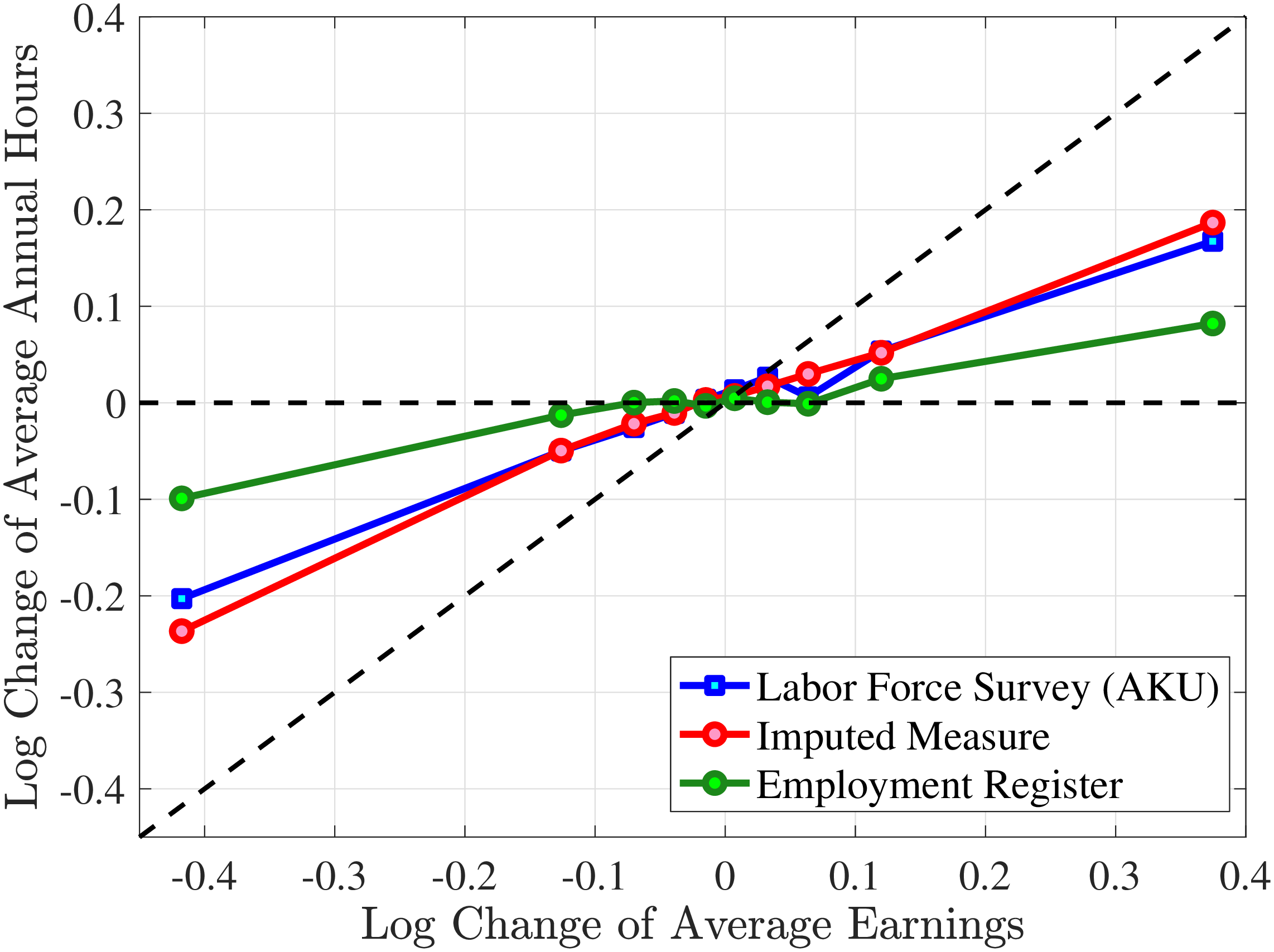
Figure 1

–

Response of Actual, Contracted, and Imputed Hours

Note: The figure displays the average one-year changes in contracted annual hours, imputed annual hours, and actual annual hours (as measured in the Labor Force Survey) for individuals with different one-year changes in annual earnings.

Figure: Figure 1 – Response of Actual, Contracted, and Imputed Hours

3.2.3 Imputing Actual Hours from Administrative Data

The downside of the Labor Force Survey data is that it has only a limited sample size, with our sample comprising about 71,000 individuals. As discussed above, all individuals present in the Labor Force Survey are also present in the register data. We merge the two data sources using individual identification numbers and design a novel imputation approach to infer actual hours worked for the entire population. We now lay out this imputation procedure, which is a contribution of independent interest.

We employ a regression tree approach to estimate actual annual hours $h_{it}^{LFS}$ from the Labor Force Survey using information from the various sources of register data as predictors. Classification and regression trees (CART) are widely used supervised machine-learning methods to develop prediction models because they are conceptually simple yet powerful.¹¹ CART algorithms are capable of handling a large number of features and observations and are easy to use. They recursively partition the training data space according to feature (predictor) thresholds into subsets with homogeneous values of the dependent variable (for example, those with earnings or hours worked above or below a certain cutoff). In the terminal nodes, the algorithm fits simple prediction models to minimize the overall mean squared error. After the tree is grown large, the algorithm then prunes some of the nodes to minimize the cross-validated sum of squares (see, e.g., Hastie et al. (2009) and Loh (2011) for further details of the machine learning algorithm).

At the terminal nodes of the tree (the leaves), we use linear regression models to minimize the errors between the measured and predicted values:¹²

\[ h_{it}^{LFS}=\beta X_{it}+\epsilon _{it}. \]

We use a rich set of regressors, $X_{it}$, from the register data (the Social Security Administration Register, the Administrative Tax and Income Records, and the Employment Register). In particular, we include contractual hours from the employment register, sickness days, parental leave days, and unemployment days reported in the Social Security Administration Register as well as their arc-percent change from last year as these are informative about total hours worked in the current year. To capture the differences in hours worked linked to job characteristics, we include indicator variables for part-time versus full-time and public versus private sector employment as well as their changes from the last year. Job change is an important predictor for labor supply (see Guvenen et al. (2019)); thus, we include indicator variables for job stayers in the current year and the last year. As is well recognized, labor supply varies over the life cycle and across education groups (see, e.g., Chakraborty et al. (2015), Bick et al. (2022)). We therefore include these variables in our set of regressors. We further include marital status and its change since last year as independent variables (see, e.g., Chakraborty et al. (2015) for variation in labor supply by marital status). Finally, we include average past earnings, current annual earnings, and arc-percent change in annual earnings as additional regressors.¹³ For details on how we construct our regressors, see Appendix A.4.¹⁴

To select the optimal regression tree structure, we experiment with various depths of the tree (up to five layers) and evaluate the goodness of fit in the training sample as well as an out-of-sample test sample. To do so, as is standard in the machine learning literature, we use 80% of our sample to fit the model and the rest to evaluate the performance out of sample. In general, choosing a deeper tree with finer categories will increase the in-sample fit, but this may come at the cost of overfitting, which will decrease the accuracy of out-of-sample predictions.

We estimate the model separately for men and women. Table I summarizes the $R^{2}$ in the training sample and test sample for different depths of the tree. For men, a regression tree of level two gives the best goodness of fit in the test sample. However, a tree with a depth of three is a very close second and performs significantly better than that of level 2 for the training sample. For women, the optimal depth level is three for the test sample. We therefore choose the tree structure with a depth of three for both men and women. Figures A.1 and A.3 show these tree structures. The associated linear-regression coefficients are reported in Tables A.3 and A.4. We use these estimated models to impute actual work hours for the individuals that are not present in the Labor Force Survey.¹⁵

The two most important covariates are contractual hours and labor earnings. The algorithm splits the sample mainly according to annual earnings and register hours for both men and women. The number of days receiving benefits for sickness, parental leave, and unemployment is also an important predictive variable. This is not surprising since the number of days on benefits is very accurately measured—it is based on actual benefit payments—whereas the number of employer-reported contractual hours in the Employment Register often misses such benefits spells. The estimations show that our model has greater explanatory power for women than for men, partly because contractual hours and earnings have a higher correlation with actual hours for women than for men.

How good is our imputation of hours worked? The explanatory power of our model is relatively high with an overall R-squared of about 0.23 for men and 0.49 for women in the out-of-sample test. This is comparable to the explanatory power of Mincer-type linear regressions on data from the PSID. Regressions on these data with annual hours worked as the dependent variable and standard covariates as explanatory variables (gender, education, a quartic in age, and, most importantly, annual earnings) yield an overall R-squared of 0.45 for women and 0.16 for men (see Online Appendix C for details).¹⁶

				Level
Depth	5	4	3	2	1	4	3	2
Wage	Yes	Yes	Yes	Yes	Yes	No	No	No
Men	28.09	26.82	25.69	24.73	23.41	22.63	21.67	20.80
Test	22.06	22.42	22.89	22.96	22.23	18.15	17.94	17.77
Women	50.65	49.65	48.79	48.08	47.21	42.79	42.06	41.31
Test	47.88	48.45	48.73	46.66	47.83	42.13	41.04	41.07

Table I – $R^{2}$ of Selected Regression Tree Models When Controlling for Change Variables

Given that our focus is to quantify the importance of hours changes for earnings risk, we investigate the average hours growth conditional on earnings changes from our imputation approach compared to those from the AKU and Employment Register data. To this end, Figure 1 plots the changes in imputed hours measure as a function of earnings changes, alongside changes in actual hours and contracted hours. Our imputed hours changes are remarkably close to the actual changes in the Labor Force Survey data. We conclude that the changes in imputed hours is a good estimate of the changes in actual hours. In the rest of the paper, we use imputed hours as our measure of annual hours worked.

We close this section with a discussion of measurement error (henceforth, m.e.) in AKU hours and imputed hours. Note first that actual hours in AKU is likely to contain m.e. both for standard reasons of survey misreporting and because our measure is constructed by multiplying hours worked in four random weeks by 13. We believe it is reasonable to assume that the m.e. in our hours variable is classical.¹⁷ Fortunately, classical m.e. in AKU hours would not affect the imputation model because it would by construction be independent of the right-hand regressors in equation (1). Second, any imputation procedure will induce some m.e. in the predicted hours relative to the true hours worked. However, we show in Section 5.2 that this m.e. in our context is of minor magnitude. Moreover, classical m.e. in imputed hours does not affect the analysis in Section 4 on nonlinear persistence because there we average over a large number of individuals, implying that the classical m.e. will wash out.¹⁸

Finally, we recognize that individuals who actually respond to any survey, including the AKU survey, will by construction be selected (as they are the ones who responded). Because we linked all AKU interviewees to the register data, we can assess the extent to which those who respond to AKU are selected relative to those who have incomplete or missing responses in AKU. Appendix Tables A.1 and A.2 document that the AKU sample has somewhat lower variance of growth in register hours and lower variance of earnings and earnings growth than the full population of men. The main reason for the lower dispersion of earnings and hours in the AKU sample is that the survey undersamples individuals with low earnings and individuals with large changes in earnings and register hours. The differences in skewness and kurtosis are small. Note that all the analysis in the paper is done on the full sample and the purpose of the AKU data is only to provide an imputation model of hours worked. We conjecture that our imputation model for hours is not significantly affected by the selection in AKU because our CART regression-tree model explicitly incorporates non-linearities associated with low earnings and low register hours. In particular, our CART model has separate branches and, hence, separate regressions at each node, for individuals with very low earnings and very low register hours.

3.3 Sample Selection and Empirical Methodology

We follow a nonparametric empirical methodology building on Guvenen et al. (2019); Guvenen et al. (2014). The idea is to group workers with similar observables at a sufficiently fine level so that they can be thought of as approximately ex ante identical. Then, for each such group, we investigate the properties of income changes as a proxy for the nature of idiosyncratic risk that individuals within that group are facing. This methodology allows us to uncover the heterogeneity in the nonnormalities and nonlinearities in earnings dynamics that different groups of workers face.

Base Sample

Our base sample is a revolving panel of 25- to 60-year-old workers with a reasonably strong labor market attachment. We first define an individual-year earnings observation as being admissible for that year if the individual (i) is between 25 and 60 years old and (ii) has labor earnings above $Y_{\text{min},t}=5\%$ of median earnings and (iii) works more than 200 (imputed) hours per year.¹⁹ Then, for each year $t$ between 2003 and 2013, we select individuals who are admissible in $t-1$ and in at least two more years between $t-5$ and $t-2$. This condition ensures that the individual has a reasonably strong labor market attachment. Given these restrictions, our sample consists of 19.9 million individual-year observations in total, which is roughly 900,000 males and 800,000 females per year.

Worker Groupings

One of the key observables we sort workers on is their recent earnings (RE) between $t-1$ and $t-5$, $\bar{Y}_{t-1}^{i}$. By requiring individuals to have at least three years of admissible income in the last five years, we ensure that we can compute a reasonable measure of each person’s average past income. We compute each individual’s RE $\bar{Y}_{t-1}^{i}$ by summing his or her annual wages normalized by age effects between $t-1$ and $t-5$: \[ \bar{Y}_{t-1}^{i}\equiv \sum _{s=1}^{5}\frac{\tilde{Y}_{t-s,h-s}^{i}}{\text{exp}(d_{h-s})}, \] where $\tilde{Y}_{t-s,h-s}^{i}$ denote the annual wage earnings of individual $i$ who is $h$ years old in year $t$. The constants $d_{h-s}$ are age dummies from regressing log individual earnings on a full set of age, gender, and cohort dummies. Next, we group workers by their gender and age in $t-1$. Within each of these groups, we rank workers into 10 deciles with respect to their recent earnings $\bar{Y}_{t-1}^{i}$.²⁰

Growth Rate Measures

We use two types of measures of growth in the variables of interest $Z$ where $Z$ is earnings, income, hours worked, or hourly wages. The first measure focuses on growth in average $\bar{Z}$ for a group of similar workers. In particular, for a group $j$ of workers who have similar observable characteristics, $V_{t+1}^{j}$ (namely, they are in the same age group, have similar recent earnings in $t-1$, and have experienced a similar earnings change between $t$ and $t+1$), we define the average growth between $t$ and $t+k$ as follows: \[ \Delta \mathrm{RA}_{t,t+k}^{Z}=\log (\bar{Z}_{t+k,h+k}^{j}\mid V_{t+1}^{j})-\log (\bar{Z}_{t,h}^{j}\mid V_{t+1}^{j}), \] where $\bar{Z}_{t,h}^{j}\equiv \sum _{i=1}Z_{t,h,i}^{j}$ and $Z_{t,h,i}^{j}$ is variable $Z$ for individual $i$ in group $j$.

We refer to this as the representative agent (RA) change. One major advantage of this approach is that it incorporates the extensive margin when going forward. For example, even though a person drops out of the labor market, the impact of his or her (zero) earnings will be included through the average change for the group. Another advantage of the representative agent change is that the persistence of the original shock to earnings is identified in a nonparametric way. Assuming that future idiosyncratic shocks to individuals in the group are independent, the future idiosyncratic innovations will wash out across group members. Therefore, the evolution of the group mean $\bar{Z}$ captures the expected evolution after the initial shock for the group. We study both short-term and long-term RA changes.

When investigating the distribution of (idiosyncratic) shocks (in Section 5), we focus instead on a measure of individual growth because we are interested in the higher-order moments of dynamics in outcomes for individuals. We work with the log growth rate in individual-specific variables between $t$ and $t+k$: {}^{k}z_{t}{i}z{t+k,h+k}^{{i}-z{}_{t,h}}{i}, where $z_{t}^{i}\equiv \log Z_{t,h}^{i}-d_{h}^{z}$ denotes the log of variable $z$ net of age effects of the same variable. This is a widely used growth rate measure, and its higher-order moments for a log-normal distribution are familiar to most readers (zero skewness and a kurtosis coefficient of 3). Recall that our sample includes observations with labor earnings above $5\%$ of median earnings. Thus, when calculating $\Delta _{\log}^{k}z_{t}^{i}$, we drop individuals from the base sample whose observations are below the cutoff in either $t$ or $t+k.$²¹

4 Dissecting Earnings Dynamics

Changes in earnings are due to changes in hours worked, changes in the hourly wage rate, or joint changes. This section documents the extent to which earnings dynamics are driven by hours versus hourly wages. The answer to this question matters for many economic questions, including risk sharing and social insurance arrangements (see, e.g.,? and?). A large literature, dating back to seminal papers by Abowd and Card (1989), MaCurdy (1981), Altonji (1986), and Abowd and Card (1989), has studied the covariance structure of changes in wages and hours. Most of the focus has been on uniform relations between movements in wages and movements in hours. However, data restrictions have so far made it difficult to examine possible heterogeneity in the covariance structure of wage and hours growth. In this paper, we exploit the sheer size of our administrative data and our novel imputation of hours to document the heterogeneity in the co-movements of hours and wage growth across individuals who experience earnings changes that are small versus large, negative versus positive, and across workers with different earnings histories.

We first quantify the importance of hours and wage changes for earnings changes, and then document how hours versus hourly wages account for the asymmetries and nonlinearities in earnings dynamics.

4.1 Decomposing Earnings Changes to Hours and Wage Growth

We measure the hourly wage rate as earnings/hours. This is the common approach in the literature (see, e.g., Heathcote et al. (2010a), Heathcote et al. (2014), Bick et al. (2022)) as wage rates are rarely directly observable in the data. We proceed by decomposing earnings changes into changes in hours worked versus hourly wages. To this end, we group them with respect to their earnings growth (in addition to conditioning workers with respect to age and recent earnings $\bar{Y}_{t-1}^{i}$).²² In particular, within each age and RE group, we rank workers on their earnings growth from $t$ to $t+1$ and sort them into 20 different quantiles. We treat each such finely defined group as homogeneous and plot the growth of their average hours and hourly wages on the y-axis conditional on their earnings growth between $t$ and $t+1$ on the x-axis.²³ To control for age effects and differences in mean reversion between different groups of workers, we normalize changes on both the x- and y-axes such that their values at the median quantile cross at zero.

In Figure 2, we start with the 40% of prime-age males (36-55 years old) who are in the middle of the recent earnings distribution (i.e., the 4th to 7th deciles). The differences across these deciles are negligible. Note first that for large negative earnings changes, hours growth is roughly as large as wage rate growth. For example, the group of workers whose earnings decline around 60 log points on average experience a decline of about 30 log points in hours and a decline of 30 log points in wage rates. For large positive changes, the hourly wage rate increases slightly more than hours worked. Second, small earnings changes (both gains and losses) are mainly driven by wage changes. For example, for men who experience a loss of 10 log points in earnings, more than 70% of this loss is from a decline in wage rates. These results illustrate the heterogeneity in the covariance structure of wage and hours growth over the earnings change distribution.

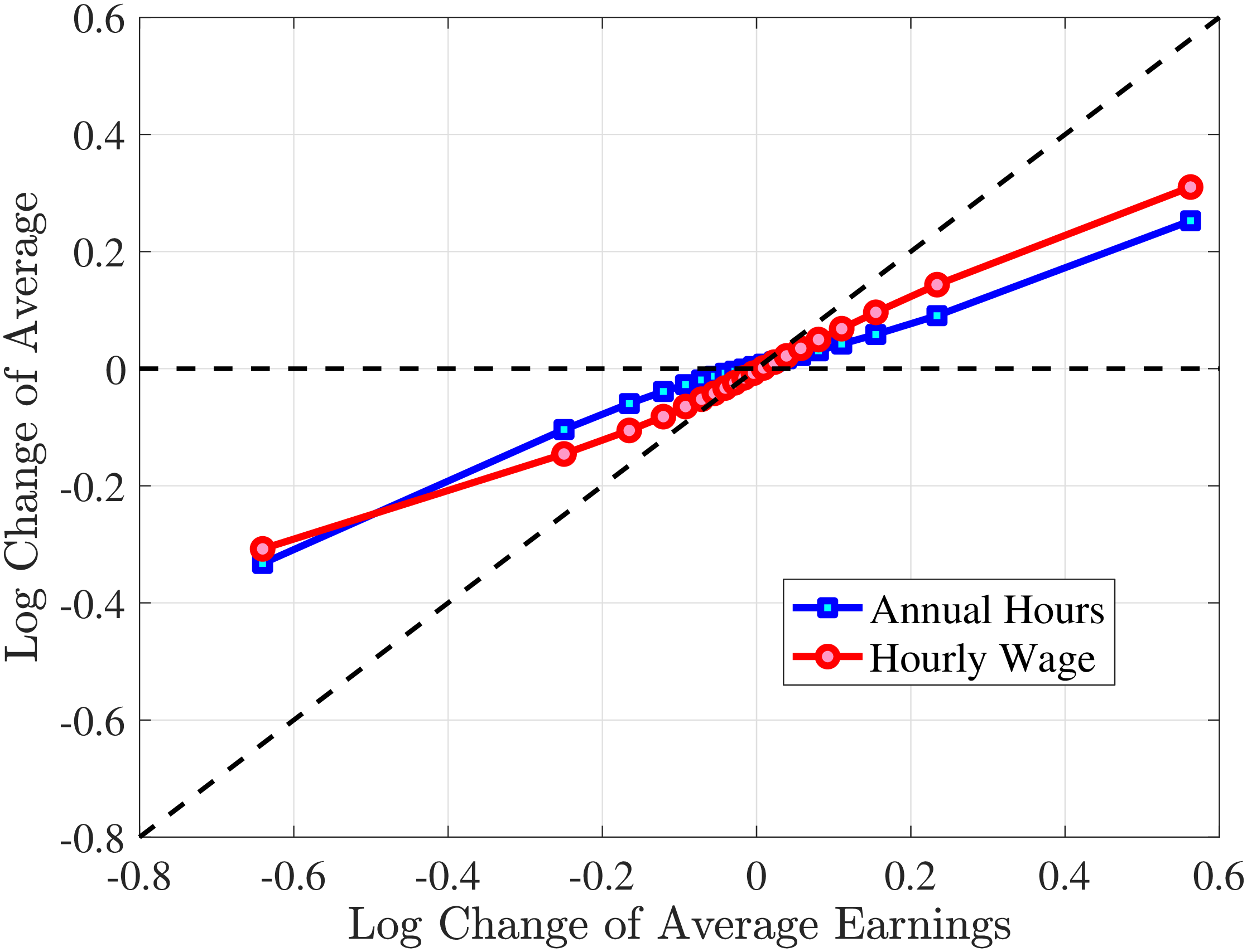
Figure 2

–

Contribution of Hours and Wages to Earnings Shocks, 4th-7th RE Deciles

Note: The figure displays the one-year representative agent change (log change of averages) for imputed hours and imputed wage rates for 20 different groups of prime-age males (ages 36 to 55) in the 4th-7th RE deciles, plotted against their contemporaneous one-year log change in average annual earnings.

Figure: Figure 2 – Contribution of Hours and Wages to Earnings Shocks, 4th-7th RE Deciles

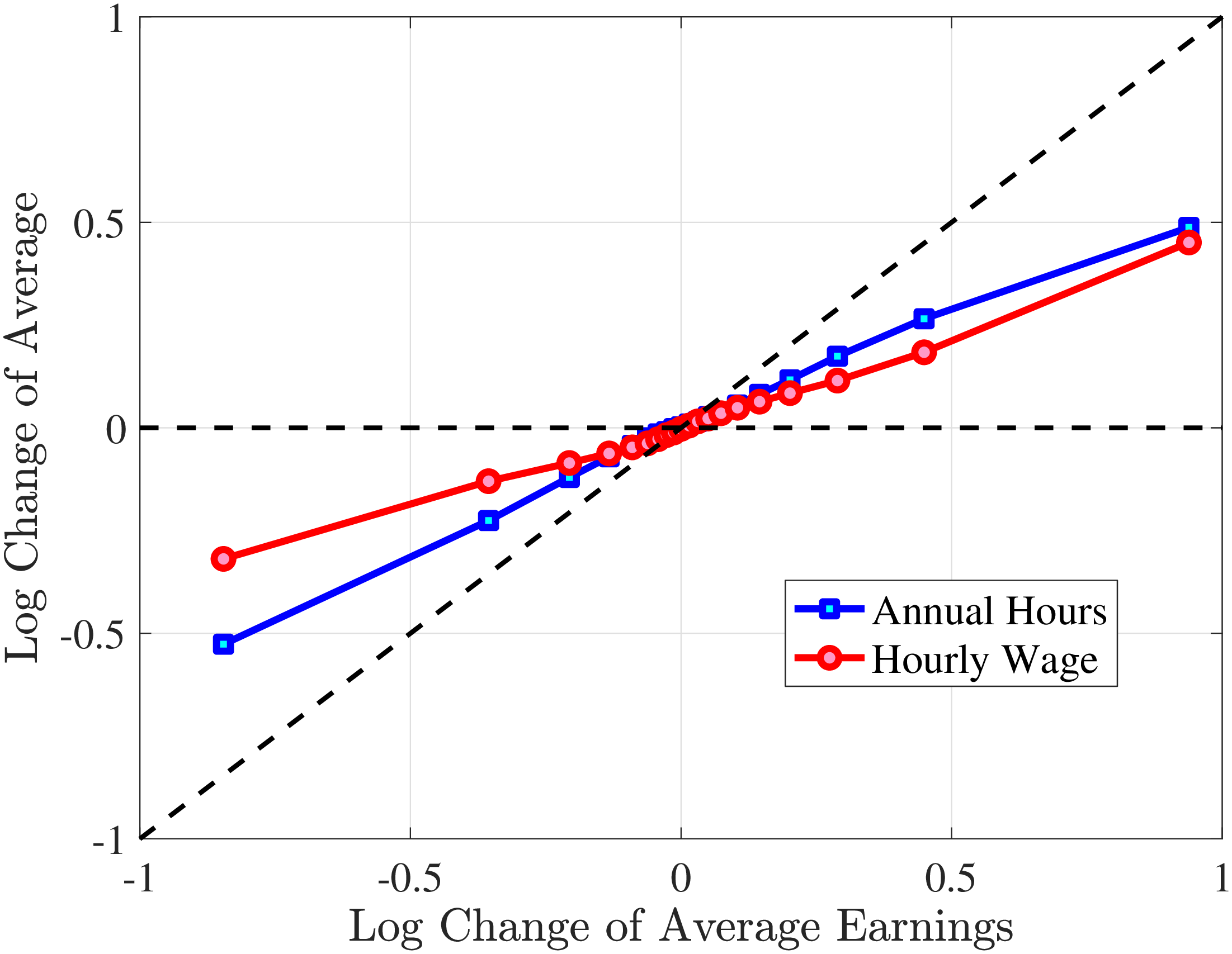
We next consider the role of hours and wage changes for the extreme ends of the recent earnings groups. Figure 3 plots the changes in hours worked and wage rates against changes in earnings for the bottom decile (left panel) and top decile (right panel) of recent earnings (see Appendix B.2 for the 2nd, 3rd, 8th, and 9th RE deciles). For the bottom decile of recent earnings, changes in hours worked are more important than changes in wage rates in accounting for earnings changes, especially for large earnings declines. This result is flipped for the top earners: high earners experience only minor changes in hours worked, and most of their earnings changes can be attributed to changes in hourly wage rates. These findings suggest that different economic mechanisms are behind the earnings dynamics of high and low earners. These results are consistent with previous research showing that unemployment risk is an important component of idiosyncratic risk for low-income workers, whereas wage fluctuations are the main drivers of income risk of workers at the higher end of the income distribution who have more stable jobs (Karahan et al. (2019)).

1st RE Decile

10th RE Decile

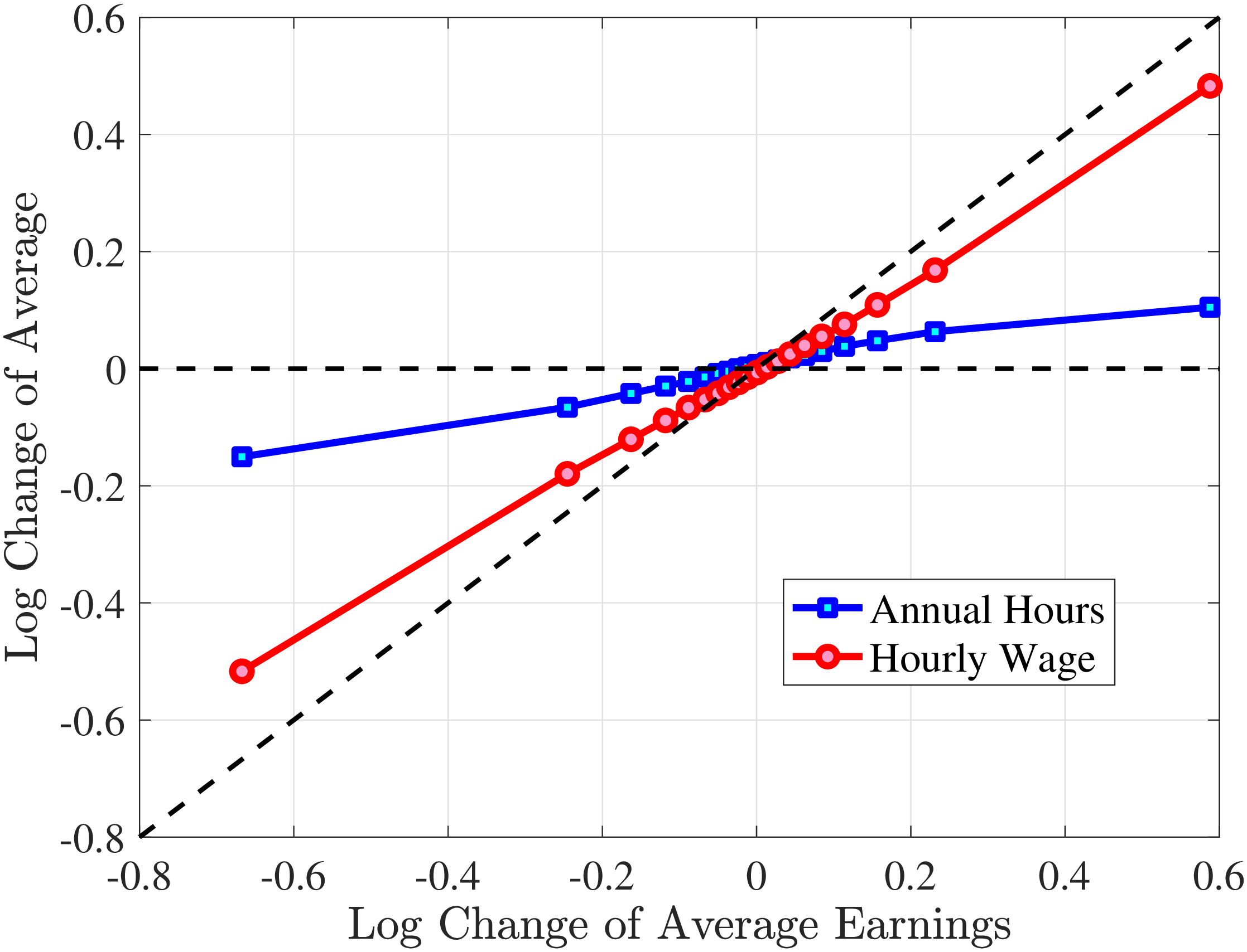
Figure 3

–

Contribution of Hours and Wage Rates to Earnings Shocks

Note: The figure displays the one-year representative agent change (log change of averages) for imputed hours and imputed wage rates for 20 different groups of prime-age males (ages 36 to 55) in the 1st RE decile (left panel) and 10th RE decile (right panel), plotted against their contemporaneous one-year log change in average annual earnings.

Figure: Figure 3 – Contribution of Hours and Wage Rates to Earnings Shocks

4.2 Asymmetric Mean Reversion

We now investigate how the persistence of earnings changes can be attributed to the dynamics of hours versus wage rates. We start by documenting how the persistence of earnings change varies by the magnitude of the change and recent earnings in Norway (e.g., Guvenen et al. (2019) and Arellano et al. (2017)). To this end, we plot the change in average earnings after five years against the initial change for prime-age males. The x-axis has the initial (average) change $y_{t+1}^{i}-y_{t}^{i}$ for each quantile of workers, sorted by the size of their earnings shock. The y-axis plots the representative agent change in earnings, that is, the change in the log of average earnings for each such quantile from $t$ to $t+5,\log \mathbb{E}\left [Y_{t+5}^{i}\right]-\log \mathbb{E}\left [Y_{t}^{i}\right]$, where $Y_{t}^{i}$ is the income level net of age and time effects of individual $i$. If the initial change were permanent, then $\mathbb{E}\left [Y_{t+5}^{i}\right]=\mathbb{E}\left [Y_{t+1}^{i}\right]$ because individual changes after $t+1$ wash out across people in the quantile. In this case, the observations would line up along the 45-degree line. Conversely, if the change between $t$ and $t+1$ were transient, then $\mathbb{E}\left [Y_{t+5}^{i}\right]=\mathbb{E}\left [Y_{t}^{i}\right]$, and the observations would line up on the x-axis. Recall that this approach incorporates changes in the extensive margin of labor supply after the initial change. While, by construction, all people in the sample satisfy the sample restrictions in periods $t$ and $t+1$, we do not impose any restriction for period $t+5$. Therefore, all individuals in the quantile, even those with zero earnings and hours, are included in $t+5$.

Consider first the workers around the median of recent earnings (4th to 7th deciles). Figure 4 reveals a striking pattern: both small changes and large positive changes are close to permanent. However, for the 10% of workers who experience the largest negative changes (i.e., reductions in earnings of more than 15%), the earnings changes are more transitory. For example, workers who experience an initial 35% decline (45 log points) in earnings relative to time $t$ have an average reduction in earnings of just 15% five years later (relative to year $t$).

For the bottom decile of RE workers, these patterns are even more pronounced: earnings losses are transitory, whereas earnings gains are, for all practical purposes, permanent. For example, workers in this group who experienced around a 55% decline (80 log points) in their earnings between $t$ and $t+1$ will on average experience earnings five years later that are only 10% less than their $t$ values. However, there is no mean reversion for either small changes or large positive changes.

Consider now the top decile of RE workers. For this group, small changes are also permanent. However, different from low-earnings workers, large positive changes are quite transient whereas large negative changes are highly persistent. For example, for the workers with initial earnings increases of 75% (55 log points), only half of the initial change remains after five years. Conversely, the workers who experience an initial 50% decline (70 log points) see a sustained 40% decline (50 log points) five years later.

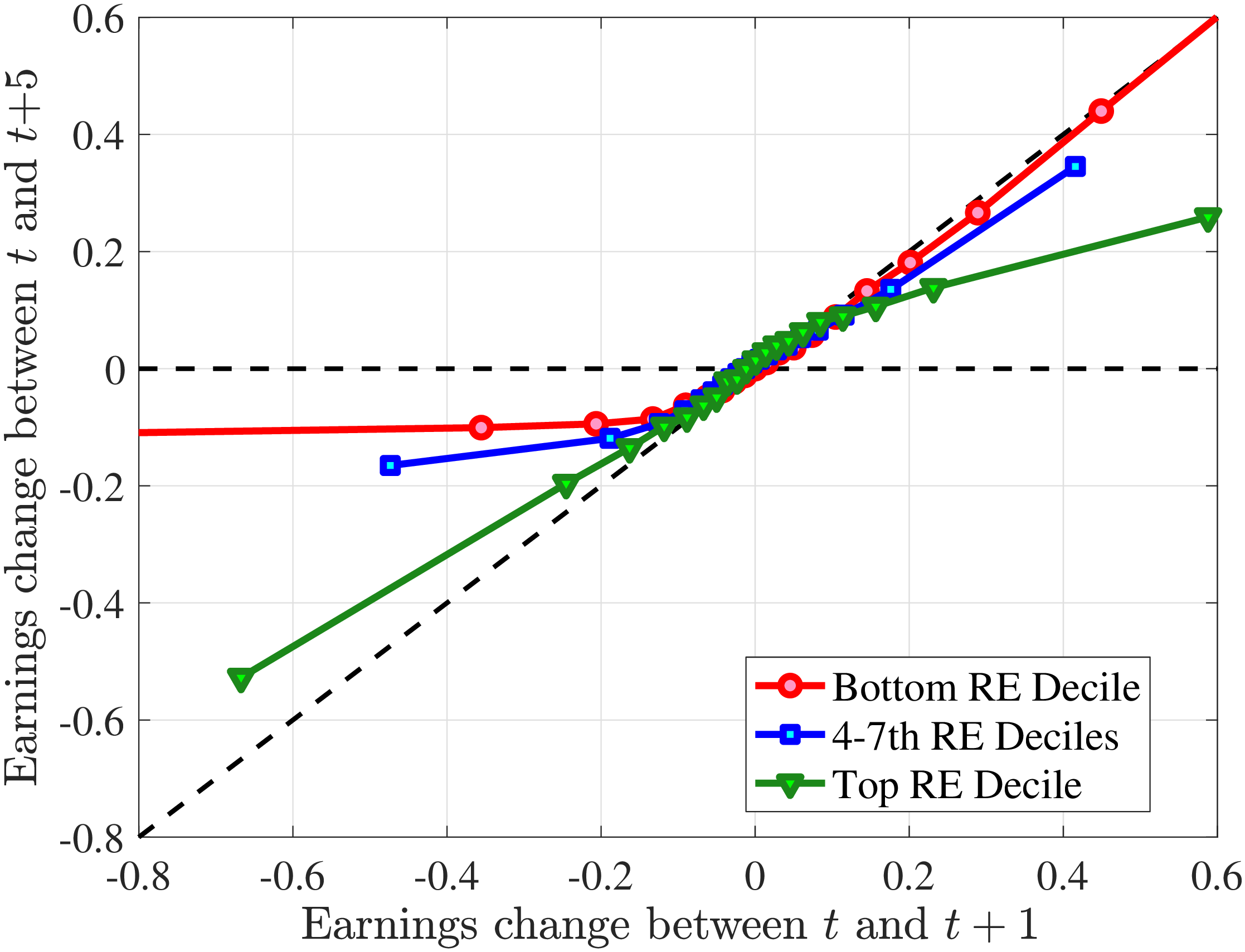
Figure 4

–

Persistence of Earnings Changes, Prime Age Males

Note: The figure displays the five-year representative agent change (log change of averages) in earnings for 20 different groups of prime-age males (ages 36 to 55) in the 1st RE decile, 4th-7th RE deciles, and 10th RE decile, plotted against their respective one-year log change in average annual earnings.

Figure: Figure 4 – Persistence of Earnings Changes, Prime Age Males

4.2.1 Mean Reversion of Hours and Wage Changes

What explains this asymmetric mean reversion for earnings? To answer this question, we investigate the persistence of hours and wage rate changes separately. In line with the strategy above, we group workers with respect to age and recent earnings as well as their hours or wage rate growth between $t$ and $t+1$. For each quantile of change in hours or wage rate, we plot the log of the five-year growth of averages within the quantile ($t$ to $t+5$) on the y-axis against the log of the one-year growth ($t$ to $t+1$) on the x-axis.

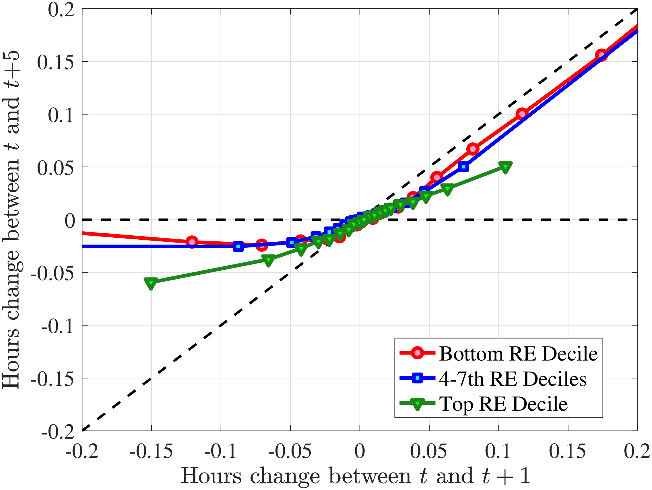
Starting with the persistence of hours change, the left panel of Figure 5 shows the five-year log change in average hours for different sizes of impulses for workers around the median of recent earnings (4th to 7th deciles), as well as those in the bottom and top deciles (similar to Figure 4). We show this graph only for the prime-age group, as young workers display a very similar pattern (see Figure D.3 in the Online Appendix). The main insights from the figure are that hours declines are very transitory, whereas hours increases are close to permanent. This finding is in line with the evidence in Krusell et al. (2011) that the duration of employment spells is much longer than the duration of unemployment spells. It is also in line with Jarosch (2021), who finds that the scarring effects of unemployment on future employment mostly dissipate after five years.²⁴

These patterns of persistence of hours—declines being mostly transitory and increases being mostly permanent—are broadly shared across income groups. The one exception is for workers in the top decile of recent earnings, for whom increases in hours become slightly less persistent and declines become somewhat more persistent. These differences might be due to different events leading to hours changes for different income groups. For example, for the bulk of workers, the main drivers of hours changes are likely to involve transitions between non-employment and employment or from part-time to full-time work, whereas for the richest workers, changes in hours might to a larger extent reflect more flexible work conditions such as the possibility of working overtime or having multiple employments. We revisit this issue in Section 4.3 when we associate earnings changes with real-life events.

The right panel of Figure 5 shows the persistence of wage rate changes. Unlike hours changes, wage rate changes are highly persistent regardless of whether they are positive or negative. We see few deviations from this pattern across recent earnings groups, although we note that large wage rate increases for top earners and large wage rate losses for bottom earners tend to be somewhat less persistent. One factor contributing to the low persistence of earnings gains for the top earners could be the fact that high earners receive some of their income in the form of bonuses and stock options, and this income is highly cyclical (c.f.?).

We conclude that the nonlinear persistence of earnings changes documented in Figure 4 is largely a result of nonlinear persistence in hours worked. In particular, hours changes exhibit nonlinear persistence patterns that are very similar to those of earnings. In contrast, wage rate dynamics are close to linear, except for workers in the tails of the income distribution. These wage rate dynamics are very different from the wage rate dynamics that one would obtain in a theoretical wage ladder model where workers climb a wage ladder within each job spell. Finally, earnings declines are very persistent for high earners because hours do not move much for these workers—the fall in their earnings is due to a decline in wage rates.

(a) Annual Hours 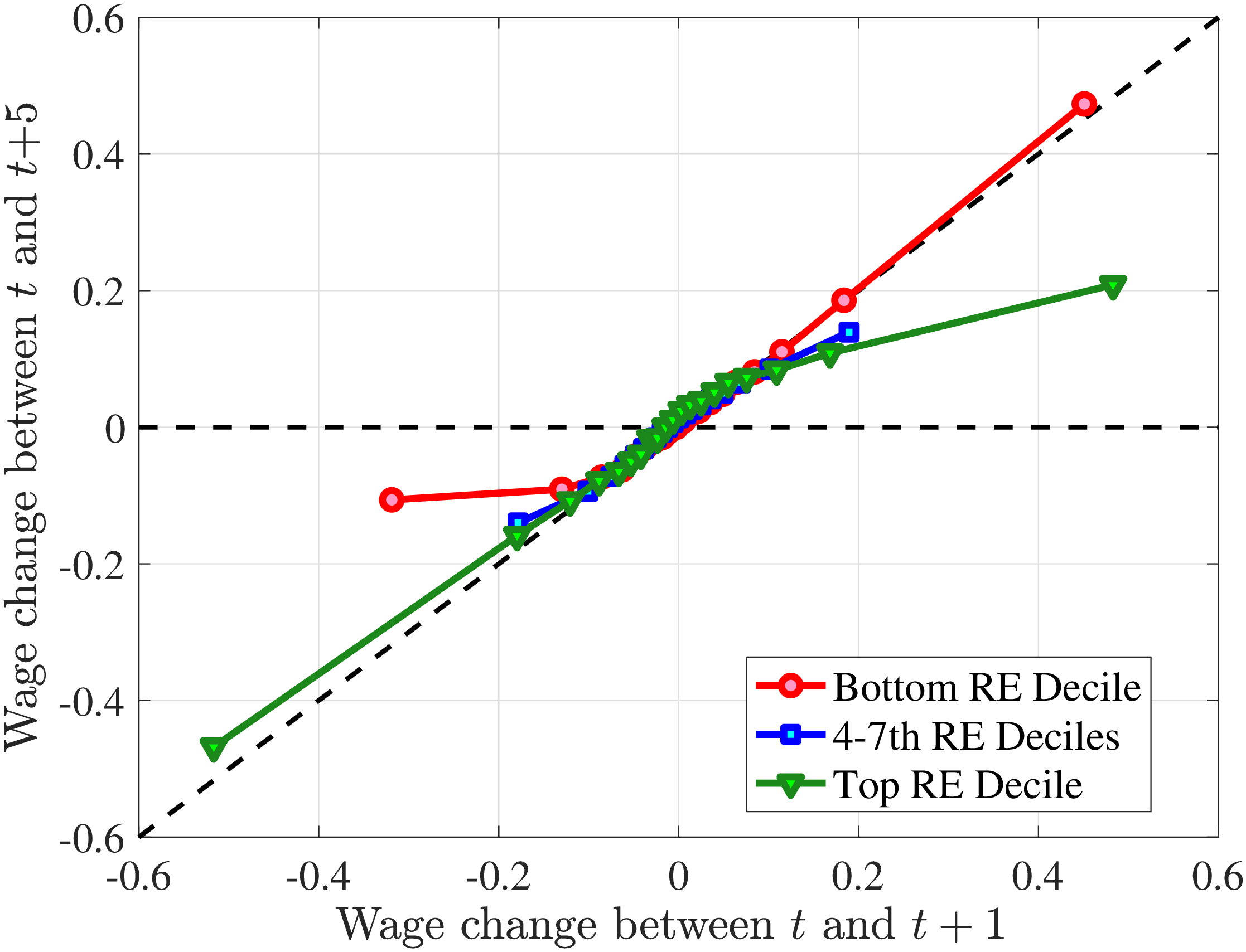(b) Hourly Wage

Figure 5

–

Persistence of Hours and Wage Changes by RE Decile

Note: The left panel displays the five-year representative agent change (log change of averages) in imputed annual hours for 20 different groups of prime-age males (ages 36 to 55) in the 1st RE decile (red line), 4th-7th RE deciles (blue line), and 10th RE decile (green line), plotted against their respective one-year log change in imputed annual average hours. The right panel displays the corresponding figure for imputed hourly wage rates.

Figure: Figure 5 – Persistence of Hours and Wage Changes by RE Decile

4.3 Life Events Associated with Large Earnings Shocks

A natural question when dissecting idiosyncratic earnings changes is, what are the major events in an individual’s life that lead to small versus large earnings changes (e.g., see?)? Our data set allows us to link individuals’ earnings to information available in other administrative data sets. In particular, we focus on five important events workers experience that are known to have significant effects on their earnings: transitioning into and out of (i) unemployment, (ii) long-term sickness, (iii) part-time work, (iv) parental leave, and (v) job change to a different firm.

We obtain data on days on unemployment benefits, sick days, and days on parental leave from the Social Security Administration Register. Transition into unemployment is defined as having zero days on unemployment benefits in year $t$ and a positive number of days on unemployment in year $t+1$. The same definition applies to days on parental benefits and number of sick days reimbursed by social security (number of days exceeding 16 days of a sickness spell). Conversely, transitioning out of unemployment, parental leave, and sickness is defined as having a positive number of days in year $t$ and zero days in year $t+1$. We obtain information on contracted work hours and main employer from the Employment Register. Transition into part-time represents changes from full-time in year $t$ into part-time in year $t+1$, where part-time is defined as 36 hours per week or less. Finally, we use the firm identifier of the main employer to construct firm change from year $t$ to $t+1$. Note that life cycle events are not mutually exclusive. A person can both become unemployed and change main employer in the same year.

We investigate the likelihood of these events in six groups of workers, sorted by the size of their earnings change between $t$ and $t+1$.²⁵ Rows (1)-(5) of Table II show the fraction of workers within each group who experience the listed five life-cycle events. In rows (6)-(9), we report the average changes in log hours and log wage rates for each group of workers on impact (between $t$ and $t+1$) and five years later (between $t$ and $t+5$). The upper panel shows the entire sample of males, and the second and third panels show the results for the bottom and top recent earnings deciles, respectively.

The events corresponding to the largest earnings changes (bigger than 50 log points, columns (1) and (6)) and the intermediate changes (between 25 to 50 log points, columns (2) and (5)) are quite similar. The only exception is that parental leave is more likely in columns (2) and (5) than it is in columns (1) and (6). As for the minor changes—the ones smaller than 25 log points—they are less likely to be associated with these events.

The most frequent cause of large losses (>50 log points) is long-term sickness, 23%, followed by change of employer, 19%, and going from full-time to part-time, 15%. Only 8% of those suffering large losses have experienced unemployment. However, an unemployment spell is on average longer than a sickness spell. The average number of weeks with sickness benefits (for males in our base sample) is around 8 weeks, whereas an average unemployment spell is 20 weeks. For those experiencing the largest earnings losses, the average decline in log hours is slightly smaller than the average log hourly wage loss: -0.40 versus -0.44. However, as discussed above, wage rate declines are substantially more persistent than hours declines. After five years, wage rates are down by 19 log points, whereas hours is only 3 log points lower.

The events behind the large positive earnings changes are relatively symmetric to the events associated with large earnings losses. The events most frequently associated with large positive changes are change of employer, 23%; going from part-time to full-time, also 23%; and returning from long-term sickness, 25%. The average change in log hours for workers with the largest positive earnings shocks is 0.40, which is somewhat smaller than the average change in the log hourly wage rate, 0.45. Increases in both hours and wages are quite persistent as well.

Overall, these patterns are similar for most income groups except for the top earners, for whom large earnings losses are to a smaller extent caused by unemployment or sickness. For the top group, large earnings losses are more closely associated with firm change than anything else. Conversely, for low-income earners, large earnings gains are chiefly associated with changes of employer and changes from part-time to full-time. The results in rows (6)-(9) of Table II confirm the findings from Figure 5 that negative shocks are transitory and positive shocks are permanent for the average worker, including the bottom decile, whereas for top earners, large negative changes in hourly wage rates are more persistent than negative changes in hours.

5 Higher-Order Earnings Risk

We now turn to the higher-order moments of individual earnings, hours and hourly wage changes. In order to investigate “transitory” and “persistent” innovations separately, it is useful to distinguish between growth over short (one-year between $t$ and $t+1$) and long (five-year from $t$ to $t+5$) horizons. The persistent component of changes becomes more salient the longer the horizon (Guvenen et al. (2019)).²⁶ In the main text, we focus on five-year changes since persistent changes are economically more important for consumption and savings behavior. The results for one-year changes are qualitatively similar (see Appendix B). In constructing the figures, we calculate the average of the moment of interest for each age/RE group over the years between 2003 and 2009.

					Annual Earnings Change, $\Delta y\in$
All		One-Year Earnings Loss			One-Year Earnings Gain
Life-cycle event		$\lt -0.5$	$[-0.5,-0.25)$	$[-0.25,0.0)$	$[0.0,0.25)$	$[0.25,0.5)$	$\geq 0.5$
into/out of		(1)	(2)	(3)	(4)	(5)	(6)
(1)	Unemployment	0.08	0.06	0.02	0.02	0.08	0.10
(2)	Long-term sickness	0.23	0.23	0.09	0.10	0.22	0.25
(3)	Part-time	0.15	0.11	0.05	0.07	0.16	0.23
(4)	Parental leave	0.06	0.08	0.04	0.05	0.08	0.05
(5)	Firm change	0.19	0.22	0.12	0.13	0.21	0.23
(6)	$\mathbb{E}\left [\Delta _{\log}^{1}h_{t}^{i}\right]$	-0.40	-0.16	-0.03	0.03	0.17	0.40
(7)	$\mathbb{E}\left [\Delta _{\log}^{5}h_{t}^{i}\right]$	-0.03	-0.03	-0.03	0.00	0.13	0.37
(8)	$\mathbb{E}\left [\Delta _{\log}^{1}w_{t}^{i}\right]$	-0.44	-0.18	-0.04	0.05	0.17	0.45
(9)	$\mathbb{E}\left [\Delta _{\log}^{5}w_{t}^{i}\right]$	-0.19	-0.15	-0.04	0.04	0.13	0.40
(10)	# of Obs.	104,727	298,777	2,219,654	1,973,893	320,891	111,353
Lowest decile (RE=1)		(1)	(2)	(3)	(4)	(5)	(6)
(1)	Unemployment	0.10	0.09	0.04	0.05	0.10	0.10
(2)	Long-term sickness	0.20	0.19	0.10	0.10	0.14	0.13
(3)	Part-time	0.16	0.12	0.06	0.13	0.25	0.32
(4)	Parental leave	0.03	0.04	0.03	0.02	0.03	0.02
(5)	Firm change	0.19	0.22	0.14	0.17	0.24	0.28
(6)	$\mathbb{E}\left [\Delta _{\log}^{1}h_{t}^{i}\right]$	-0.38	-0.16	-0.03	0.05	0.17	0.37
(7)	$\mathbb{E}\left [\Delta _{\log}^{5}h_{t}^{i}\right]$	-0.00	-0.01	-0.02	0.03	0.13	0.37
(8)	$\mathbb{E}\left [\Delta _{\log}^{1}w_{t}^{i}\right]$	-0.50	-0.19	-0.05	0.05	0.17	0.51
(9)	$\mathbb{E}\left [\Delta _{\log}^{5}w_{t}^{i}\right]$	-0.05	-0.06	-0.01	0.06	0.13	0.58
(10)	# of Obs.	17,813	22,993	124,680	145,885	39,418	37,547
Top decile (RE=10)		(1)	(2)	(3)	(4)	(5)	(6)
(1)	Unemployment	0.05	0.02	0.00	0.00	0.02	0.10
(2)	Long-term sickness	0.08	0.09	0.05	0.05	0.08	0.25
(3)	Part-time	0.15	0.11	0.06	0.06	0.11	0.23
(4)	Parental leave	0.05	0.08	0.05	0.06	0.08	0.05
(5)	Firm change	0.31	0.24	0.13	0.12	0.21	0.23
(6)	$\mathbb{E}\left [\Delta _{\log}^{1}h_{t}^{i}\right]$	-0.18	-0.09	-0.02	0.03	0.08	0.16
(7)	$\mathbb{E}\left [\Delta _{\log}^{5}h_{t}^{i}\right]$	-0.03	-0.03	-0.02	0.00	0.04	0.10
(8)	$\mathbb{E}\left [\Delta _{\log}^{1}w_{t}^{i}\right]$	-0.67	-0.25	-0.06	0.05	0.26	0.64
(9)	$\mathbb{E}\left [\Delta _{\log}^{5}w_{t}^{i}\right]$	-0.50	-0.23	-0.05	0.04	0.14	0.30
(10)	# of Obs.	15,274	34,208	310,628	298,130	32,251	11,015

Table II – Important Life Cycle Events Associated with Earnings Changes

Figure 6 displays the distribution of one-year (left panel) and five-year (right panel) individual earnings growth for male workers in the base sample defined in Section 3.3, along with Gaussian densities with the same standard deviation as in the data. The earnings growth distribution displays left (negative) skewness and excess kurtosis relative to a Gaussian density. In other words, workers face an earnings change distribution with a slightly longer left tail relative to the right tail, and there are far more people with very small and very large changes and fewer people with intermediate changes. Note that the deviations from normality are larger for one-year changes than for five-year changes. These qualitative properties are in line with findings for many other countries.

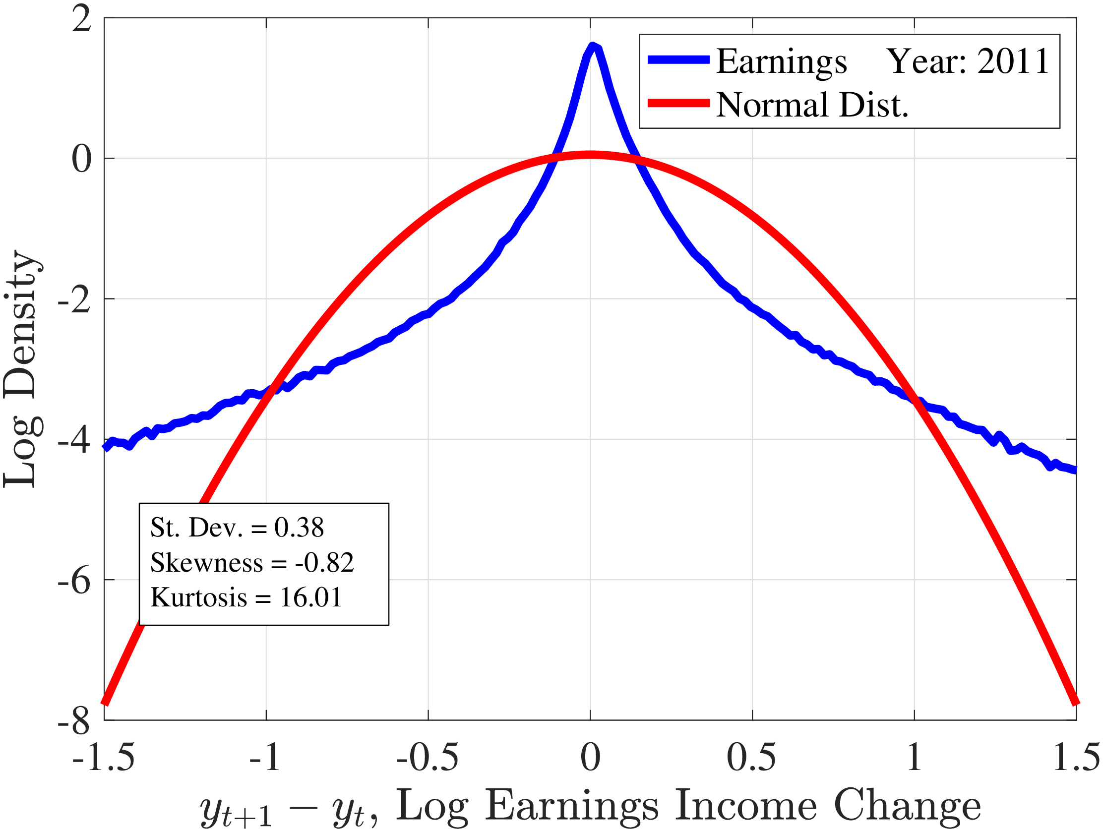
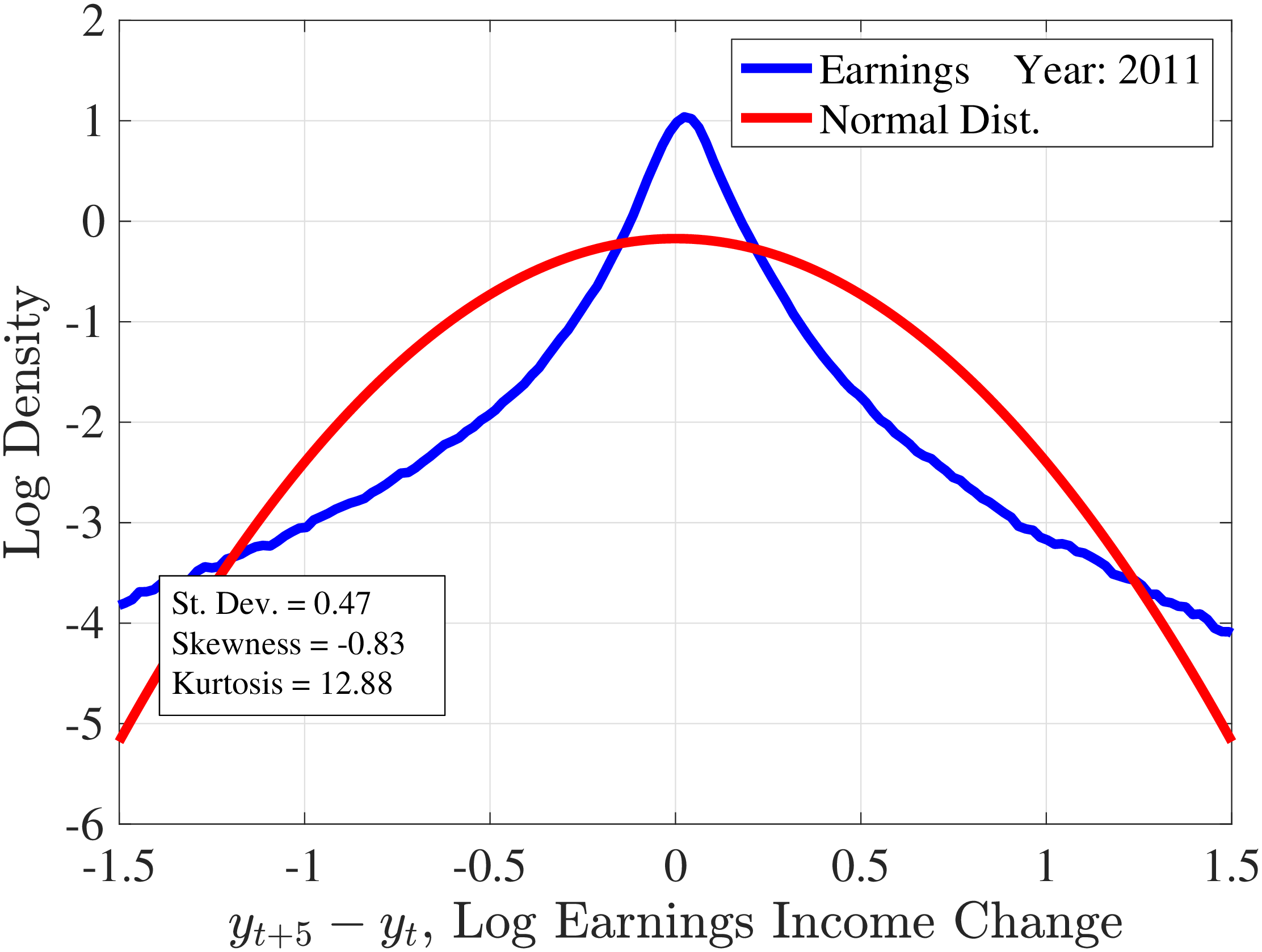
Figure 6

–

Histograms of One- and Five-Year Log Earnings Changes

Note: The figure plots the empirical densities of one- and five-year earnings changes superimposed on Gaussian densities with the same variance. The data are for male workers in the base sample defined in Section 3 and $t=2011$.

Figure: Figure 6 – Histograms of One- and Five-Year Log Earnings Changes

5.1 Higher-Order Moments for Male Earnings Growth

We now document the higher-order moments of earnings growth in Norway. Appendix B.1 contains analogous results for the U.S. as well as results for one-year earnings growth in Norway.²⁷ For comparability with earlier work, we focus on men. The results for women are reported in Appendix E. Our measure of skewness is the third standardized moment (i.e., $\operatorname{Skew}[X]=\sum _{i}^{N}\left (X_{i}-\bar{X}\right)^{3}/[(N-1)*\sigma ^{3}]$), and our measure of kurtosis is the fourth standardized moment (i.e., Pearson’s kurtosis, $\operatorname{Kurt}[X]=\sum _{i}^{N}\left (X_{i}-\bar{X}\right)^{4}/[(N-1)*\sigma ^{4}]$).

(a) Variance 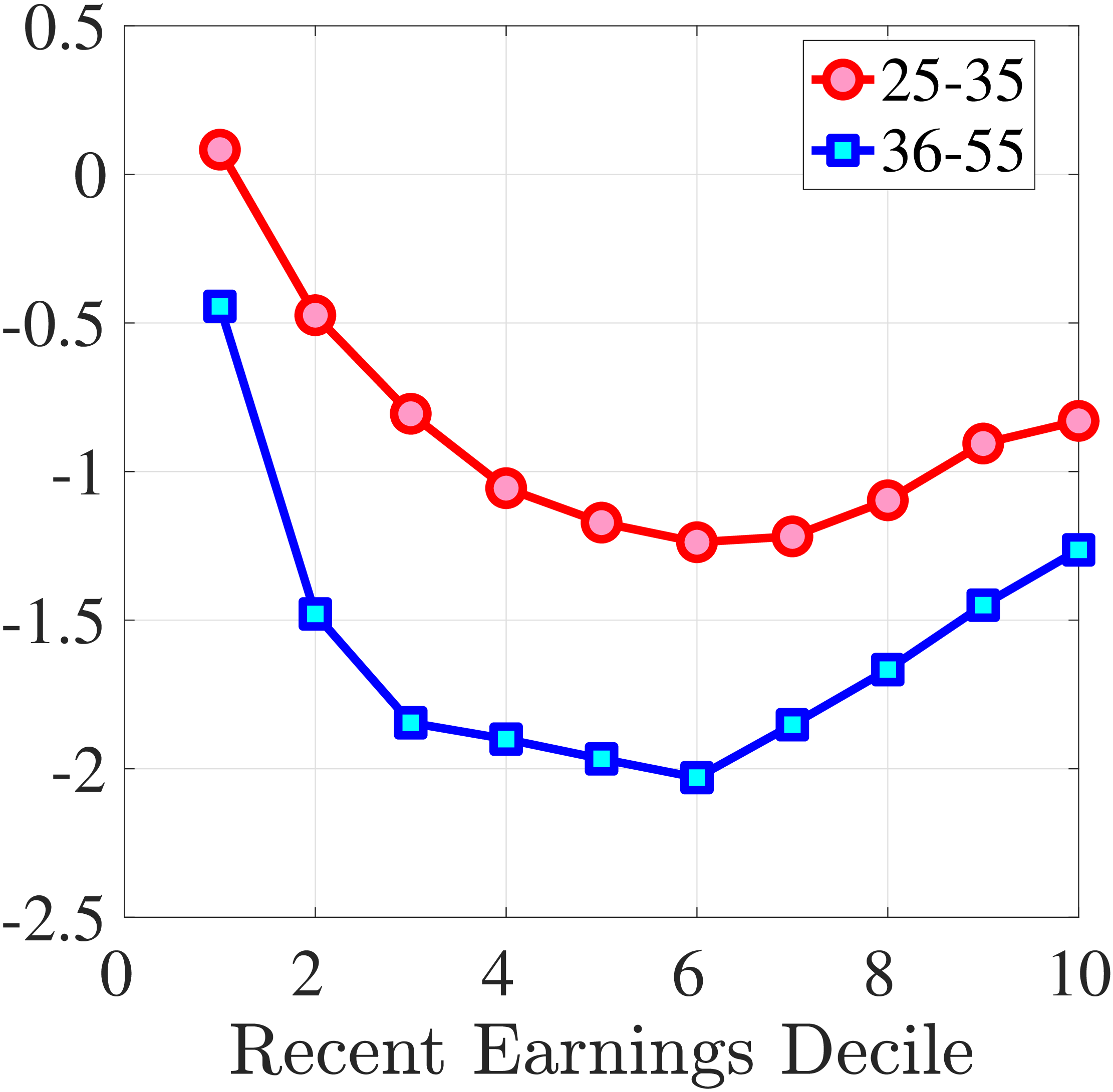(b) Skewness 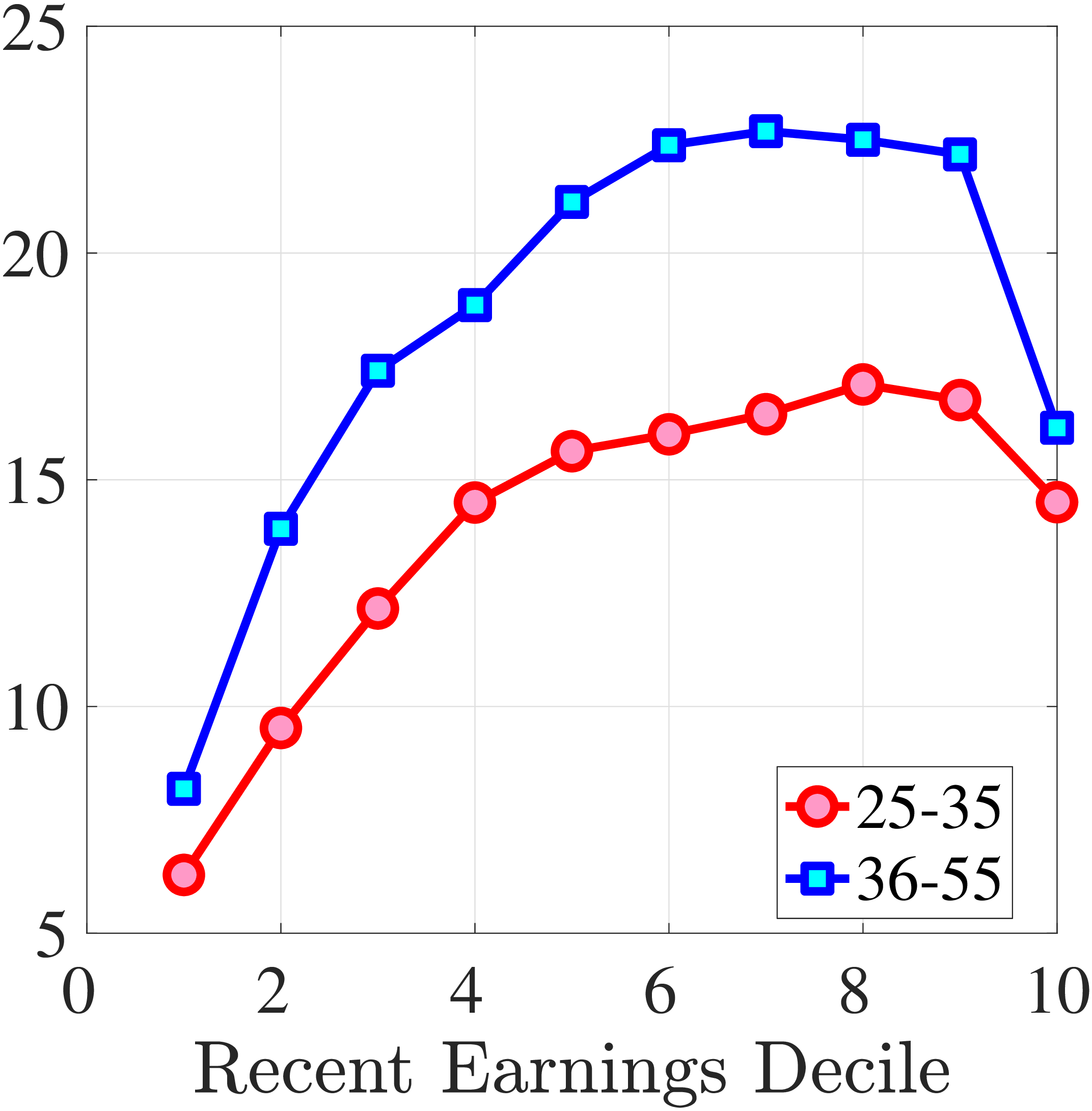(c) Kurtosis

Figure 7

–

Cross-Sectional Moments for Five-Year Earnings Growth in Norway

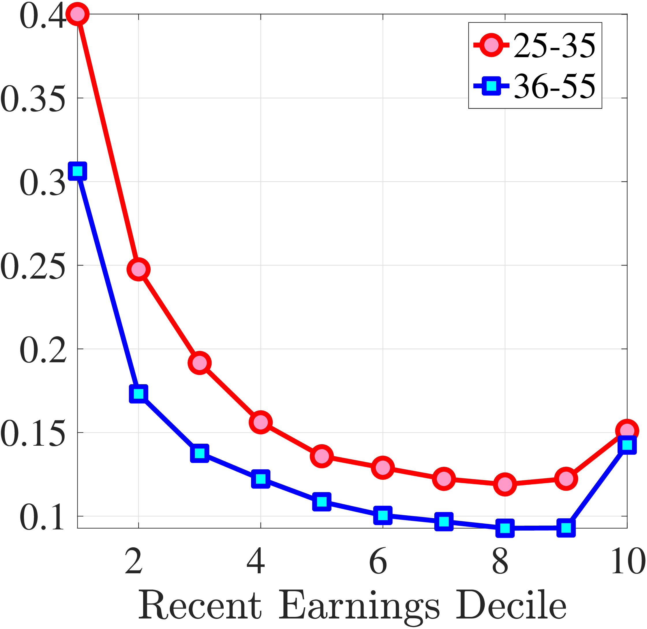
Note: The figure displays the higher-order moments of five-year log earnings changes ($y_{t+5}-y_{t}$) for young males (red line) and prime-age males (blue line) for each decile of RE.

Figure: Figure 7 – Cross-Sectional Moments for Five-Year Earnings Growth in Norway

Starting with the second moment, Figure 7 shows the variance of five-year earnings growth between $t$ and $t+5$ conditional on workers’ age and RE in $t-1$. Workers differ significantly in the dispersion of earnings growth they face with respect to their RE. In particular, for prime-age workers, the variance declines monotonically from around 0.30 for the bottom decile of RE to roughly 0.09 for the 90th percentile, after which it increases to 0.14. The life-cycle variation is smaller than the differences across RE groups, with the variance of shocks being largest for the young workers (ages 25-35). These patterns are qualitatively similar to those found for the U.S., although the variance of earnings growth is substantially smaller in Norway (Figures B.1 and B.2).

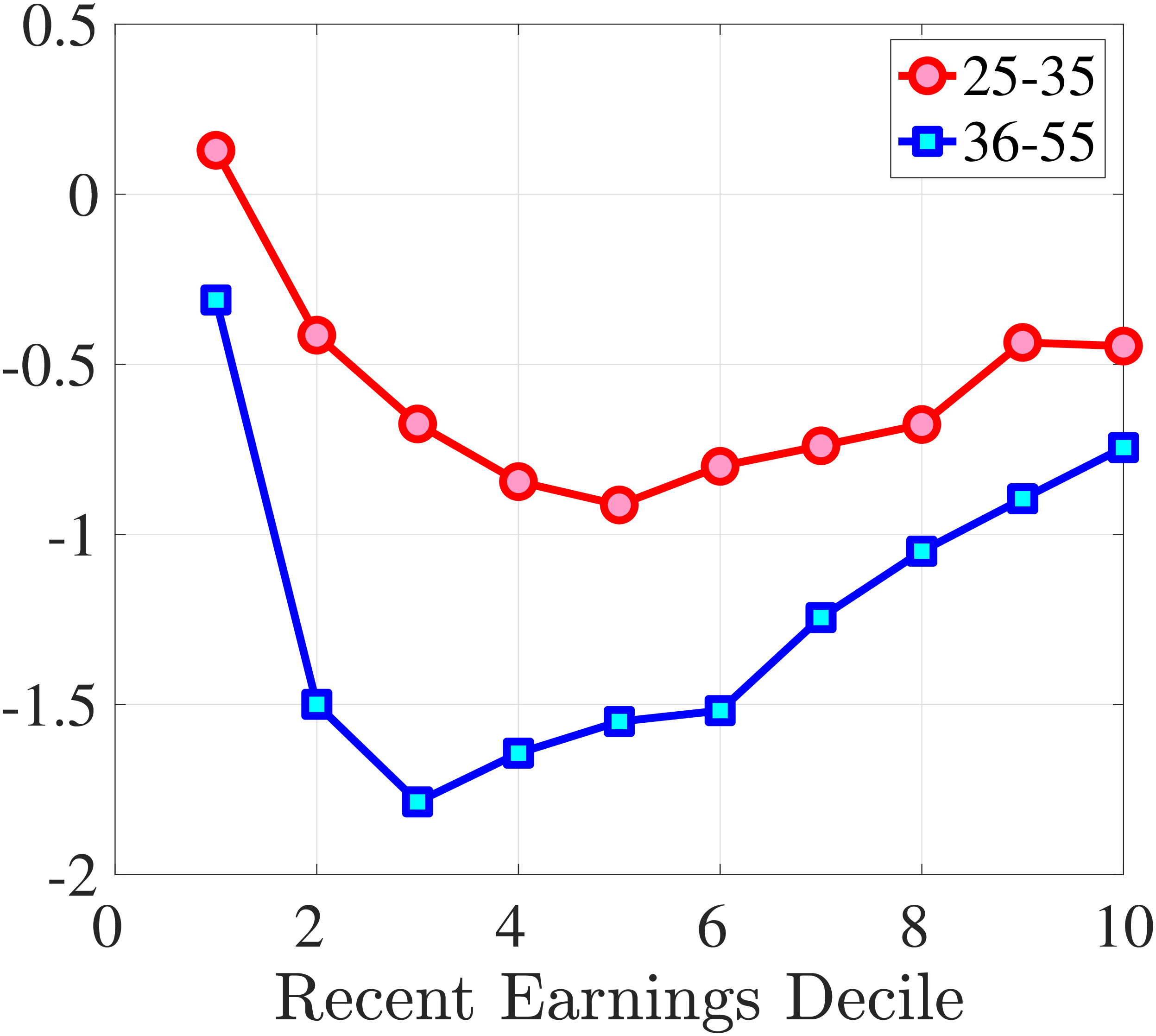
Next, Figure 7 shows that almost all male workers face a left-skewed distribution of five-year log earnings growth regardless of their RE and age, meaning that experiencing very large declines in earnings is more likely than seeing very large increases.²⁸ However, skewness is more negative for prime-age workers.²⁹ Thus, the older an individual gets or the higher his current earnings, the more gradual will be the upward movements and the more drastic will be the fall in earnings. These skewness patterns for earnings changes are similar to those documented for the U.S.

Figure 7 plots the fourth standardized moment of five-year earnings growth by age and RE. This kurtosis measure increases from around 8 for the bottom earners to more than 20 for workers with recent earnings above the median. The high kurtosis suggests that most workers experience negligible shocks, whereas a few workers experience large ones. Moreover, this asymmetry increases with age and tends to increase with recent earnings. Finally, the RE and age variations in the kurtosis of annual earnings growth in Norwegian data are similar to those documented for the U.S.

5.2 Distributions of Wage and Hours Growth

In this section, we study the extent to which the distributions of hours and wage growth display non-Gaussian features and investigate their roles in the higher-order moments of earnings. We follow a similar graphical methodology as in Section 5.1 and present the cross-sectional moments of hours and wage growth conditional on 3 age groups and 10 deciles of recent earnings.

Second Moment: Variance

Figure 8 shows the variance of changes in hourly wage rates (panel A) and hours (panel B) over the life cycle and across the recent earnings distribution. Panel C documents the decomposition of the variance of earnings changes into hours changes and hourly wage changes along with their covariance. The way the variance of both the wage rate and hours changes vary with age and recent earnings are qualitatively similar to those of annual earnings growth (panel C in Figure 8) in that the volatility of both hours and wage rate changes is falling with age. Moreover, lower-income workers tend to face a more dispersed distribution of wage rate and hours growth relative to higher-income workers. However, for recent income above the median, the patterns differ for hours versus hourly wages: the variance of changes in hours worked is monotonically falling in recent income, whereas the variance of wage rate growth is U-shaped in recent earnings, weakly increasing for groups with RE above the median. This suggests that the increasing part of the U-shaped profile of the variance of earnings growth across RE groups in Figure 7 is a result of wage rate growth becoming more volatile for the top earners. This is consistent with the view of, for example, Parker and Vissing-Jo rgensen (2010), who argue that the earnings volatility of high earners is affected by a performance-based compensation structure such as bonuses and stock options.

For workers below the median recent earnings, changes in hours and changes in wage rates are approximately equally volatile, whereas for workers at or above the median recent earnings, wage rates are more volatile than hours. The relatively volatile hours worked for poor workers might reflect that unemployment shocks are more relevant for this group. That wage rates are, broadly speaking, more volatile than hours is consistent with Heathcote et al. (2014), who document that changes in wage rates are slightly larger than changes in hours worked in the PSID. It is also consistent with the evidence from Section 4.1 that earnings changes for high earners tend to be driven by changes in wage rates rather than hours.

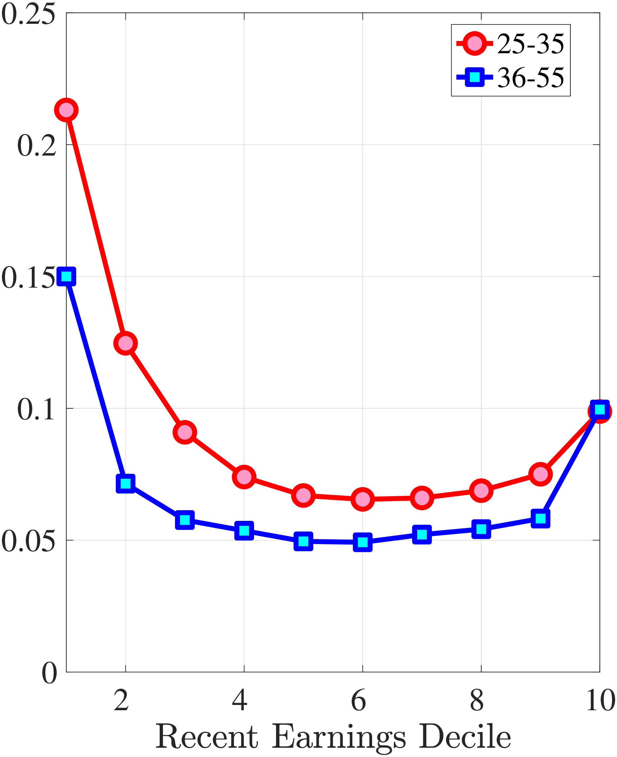(a) Variance $\Delta _{\log}^{5}w_{t}^{i}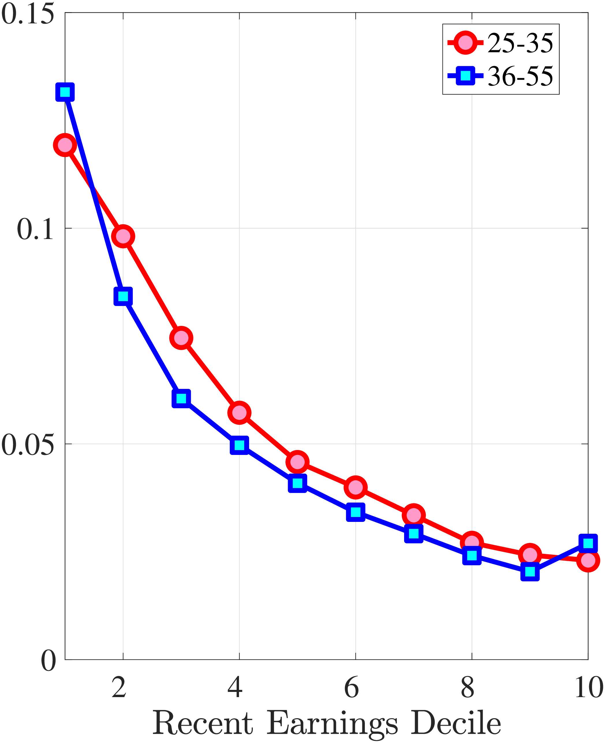$ (b) Variance $\Delta _{\log}^{5}h_{t}^{i}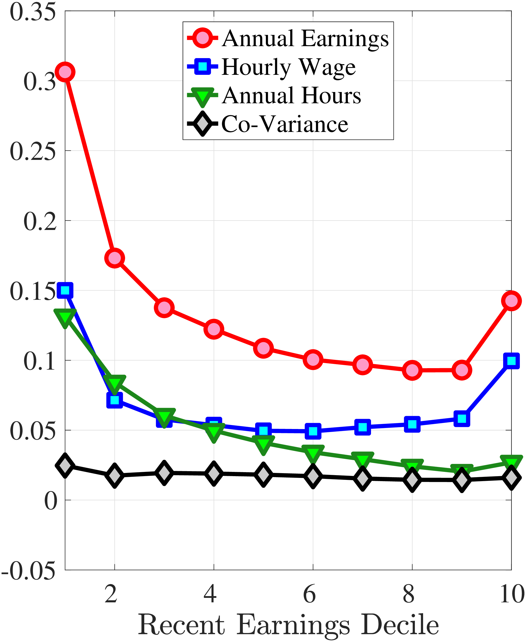$ (c) Decomposing $Var(\Delta _{\log}^{5}y_{t}^{i})$

Figure 8

–

Variance of Five-Year Log Hourly Wage and Hours Growth

Note: The figure plots the variances of five-year wage rate changes (pane A) and hours changes (panel B) by RE decile for young men (red line) and prime-age men (blue line). Panel C shows a decomposition of the variance of earnings changes into changes in hours, hourly wages, and their covariance for prime-age men (36-55 years old).

Figure: Figure 8 – Variance of Five-Year Log Hourly Wage and Hours Growth

Panel C in Figure 8 illustrates that the variance of five-year earnings growth for prime-age workers is higher than the variance of both hours growth and wage growth (see Appendix B.4 for a similar decomposition for young workers). Note that the covariance between hours growth and wage rate growth is small but positive. This positive co-movement is in line with our findings in Section 4.1. This is an important result for two reasons. First, a positive correlation between changes in hours and hourly wage rates tends to mitigate the welfare costs of (an exogenous) volatility of hourly wages. The reason is that if the correlation between changes in wage rates and changes in hours is positive, hourly wage rate changes tend to increase average productivity and average wages (see Heathcote et al. (2009) for an analysis of the aggregate welfare effects of wage rate volatility when labor supply is endogenous). In contrast, Heathcote et al. (2014) document that for U.S. workers (based on data from from PSID), hours changes and wage rate changes are negatively correlated. Second, wage-hours correlation is informative about the presence of m.e. in our imputed hours. Recall that we measure hourly wages as earnings divided by imputed hours. Classical m.e. in imputed hours will therefore give rise to a division bias lowering the measured covariance between hourly wages and hours.³⁰ The fact that we find a positive correlation between imputed hours changes and wage rate changes suggests that m.e. in our imputation of hours worked must be of minor magnitude.

Higher-order moment decomposition. The skewness and kurtosis of earnings growth can be decomposed into hours and wage components as shown in the following lemma.

Lemma 1. If x and y are two random variables, then

\[ \begin{aligned} \text{skew}\left (x+y\right) &= \left (\frac{std\left (x\right)}{std\left (x+y\right)}\right)^{3}\cdot \text{skew}\left (x\right)+\left (\frac{std\left (y\right)}{std\left (x+y\right)}\right)^{3}\cdot \text{skew}\left (y\right)\\ &\quad + \underbrace{\frac{3}{\left (std\left (x+y\right)\right)^{3}}\left (cov\left (x^{2},y\right)+cov\left (x,y^{2}\right)-2\left (E\{y\}+E\{x\}\right)\cdot cov\left (x,y\right)\right)}_{\text{co-skewness terms}} \end{aligned} \]

\[ \begin{aligned} \text{kurt}\left (x+y\right) &= \left (\frac{var\left (x\right)}{var\left (x+y\right)}\right)^{2}\text{kurt}\left (x\right)+\left (\frac{var\left (y\right)}{var\left (x+y\right)}\right)^{2}\text{kurt}\left (y\right)\\ & \underbrace{\begin{array}{cc} + & \frac{4}{\left (var\left (x+y\right)\right)^{2}}\left [E\left \{\left [x-E\left (x\right)\right]^{3}\left [y-E\left (y\right)\right]\right \} +E\left \{\left [x-E\left (x\right)\right]\left [y-E\left (y\right)\right]^{3}\right \} \right]\\ + & \frac{6}{\left (var\left (x+y\right)\right)^{2}}E\left \{\left [x-E\left (x\right)\right]^{2}\left [y-E\left (y\right)\right]^{2}\right \} \end{array}}_{\text{co-kurtosis terms}} \end{aligned} \]

See Appendix A for the derivation.

This lemma shows that the skewness (kurtosis) of the sum of two random variables is equal to the weighted sum of skewness (kurtosis) of individual variables plus some co-skewness (co-kurtosis) terms. The weights are determined by the ratio of the variance of individual variables to the variance of the sum. Thus, the more volatile variable will account for a larger share of the moments for the sum of the variables. A negative (positive) co-skewness indicates that both variables tend to undergo extreme negative (positive) deviations at the same time. Similarly, if two random variables exhibit a high level of co-kurtosis, they tend to undergo extreme deviations concurrently.

Third Moment: Skewness

Figure 9 documents the third moment of hours and wage rate growth. Again, the age and income variations in their skewness of five-year changes are qualitatively similar to those of annual earnings growth in Figure 7. First, the skewness of hours and wage rates follow a U-shaped pattern over the RE distribution, with middle RE workers facing a more left-skewed distribution of five-year wage and hours changes. Second, the distributions of five-year growth in both wage rates and hours are more left (negatively) skewed for prime-age workers relative to younger workers. Note that hours changes are more negatively skewed than wage rate changes.

(a) Skewness of Hourly Wage Changes, $\Delta _{\log}^{5}w_{t}^{i}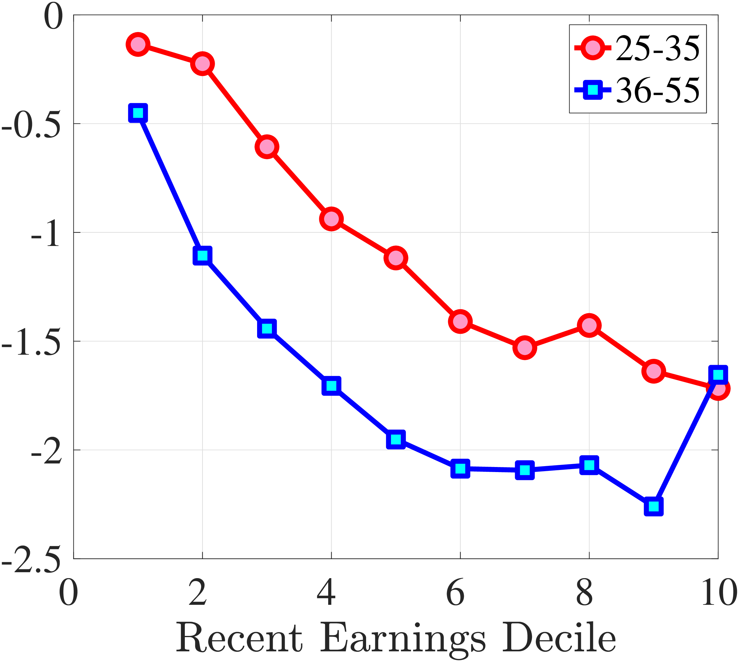$ (b) Skewness of Hours Changes, $\Delta _{\log}^{5}h_{t}^{i}$

Figure 9

–

Skewness of Five-Year Log Hourly Wage and Hours Growth

Note: The figure plots the skewness of five-year wage rate changes (left panel) and hours changes (right panel) by RE decile for young men (red line) and prime-age men (blue line).

Figure: Figure 9 – Skewness of Five-Year Log Hourly Wage and Hours Growth

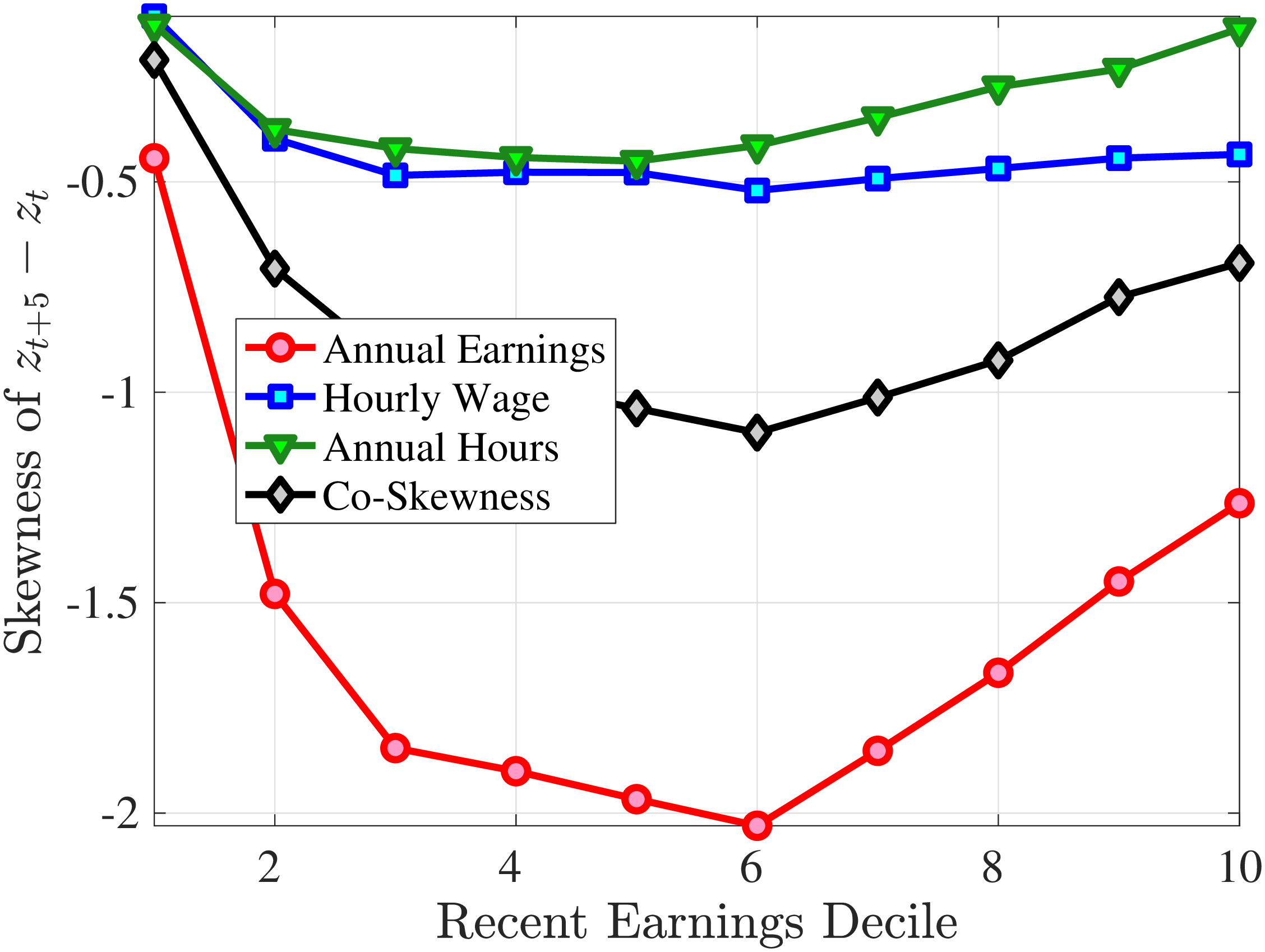
We next decompose the skewness of the earnings growth distribution into hours and wage growth components as well as the co-skewness term as defined in Lemma 1 (the left panel of Figure 10). Recall that hours and wage growth contribute to the skewness of earnings growth according to the ratio of their variance to the variance of earnings growth. Thus, even though hours growth is more left skewed than wage rate growth, the fact that wage rate growth is more volatile implies that it accounts for a larger share of the left skewness of earnings growth, especially for groups with RE above the median. More importantly, the main driver of the left skewness of the earnings changes are the co-skewness terms. This component captures the fact that hours and wages tend to undergo large negative changes simultaneously, in line with the evidence in Figures 2 and 3. Thus, when workers experience large hours cuts, they also see their wages decline sharply. This finding is consistent with the literature studying the labor market dynamics associated with unemployment, where large initial declines in hours are associated with large and persistent declines in earnings (e.g., Jacobson et al. (1993); Von Wachter et al. (2009), and Huttunen et al. (2011) for Norway). However, our results from Section 4.2.1 suggest that the scarring effect of unemployment takes the form of an initial fall in hours and wage rates, followed by almost full recovery in hours but little recovery in wage rates.

(a) Skewness 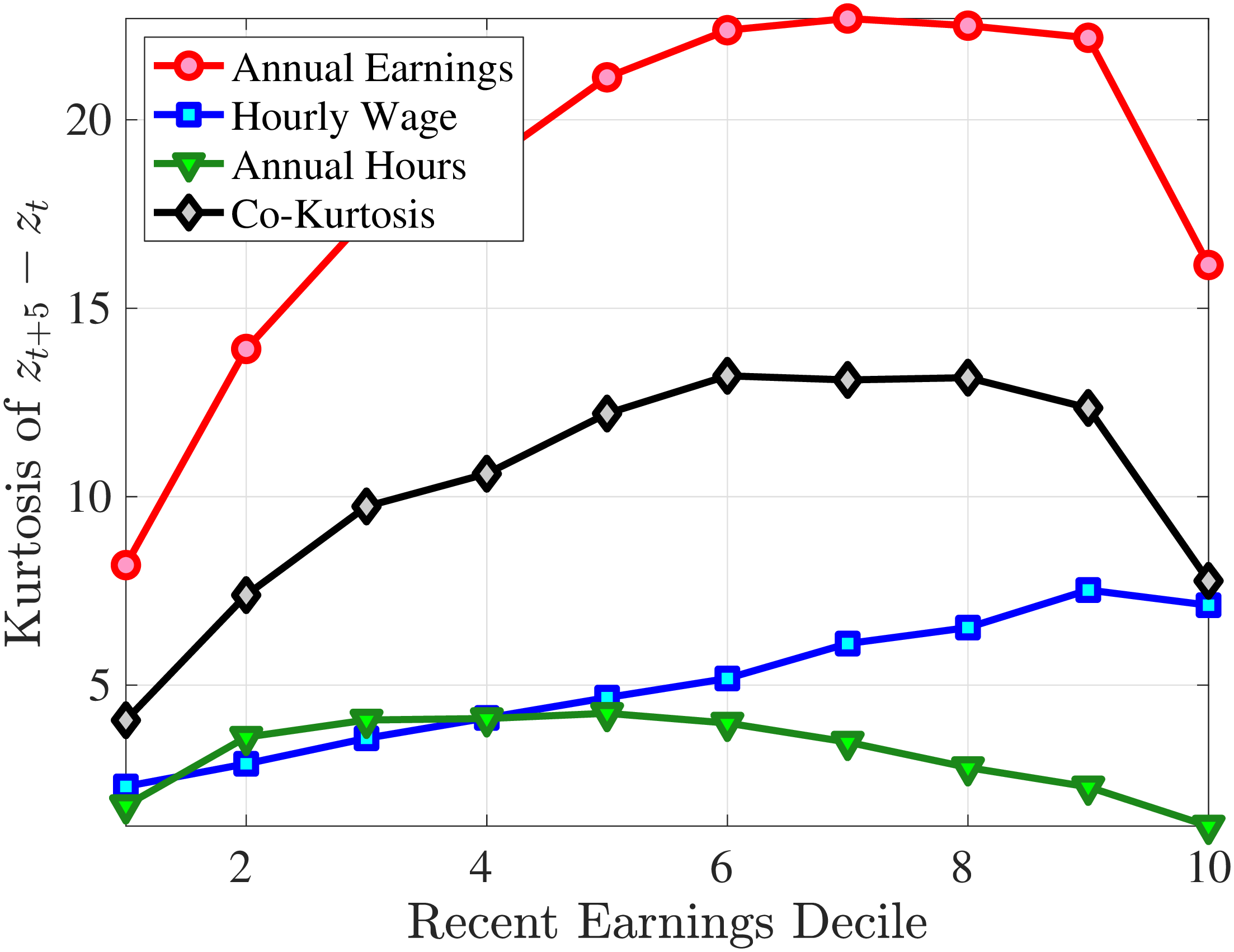(b) Kurtosis

Figure 10

–

Decomposition of Skewness and Kurtosis of Five-Year Log Earnings Growth

Note: The figure plots a decomposition of skewness (left panel) and kurtosis (right panel) of five-year log earnings changes (red line) for prime-age men into the skewness/kurtosis of log wage changes (blue line), the skewness/kurtosis of log hours changes (green line), and the co-skewness/co-kurtosis between log wage and log hours changes (black line). Each dot represents a decile of RE. The decomposition is based on Lemma 1.

Figure: Figure 10 – Decomposition of Skewness and Kurtosis of Five-Year Log Earnings Growth

Fourth Moment: Kurtosis

Finally, Figure 11 shows the income and age profiles of the fourth standardized moment of five-year wage (left panel) and hours growth (right panel). Both variables display very large excess kurtosis. The kurtosis of wage rate changes and how it varies with age and recent earnings groups are very similar to those of earnings growth (Figure 7). The kurtosis of hours growth is significantly higher than the kurtosis of wage and earnings growth. Thus, hours changes are less frequent but more extreme, so when they change, the changes are large. Furthermore, the kurtosis of hours changes also displays an increasing profile over the RE distribution, compared to a hump-shaped profile for the kurtosis of wage changes. As for the age variation, older workers are facing more leptokurtic hours, and their wage growth distributions are similar to the distribution of earnings changes. These features of hours changes are broadly consistent with transitions into or out of unemployment or part-time work for prime-age male workers. Such flows feature infrequent but large changes in hours, especially, for those at the higher end of the RE distribution.

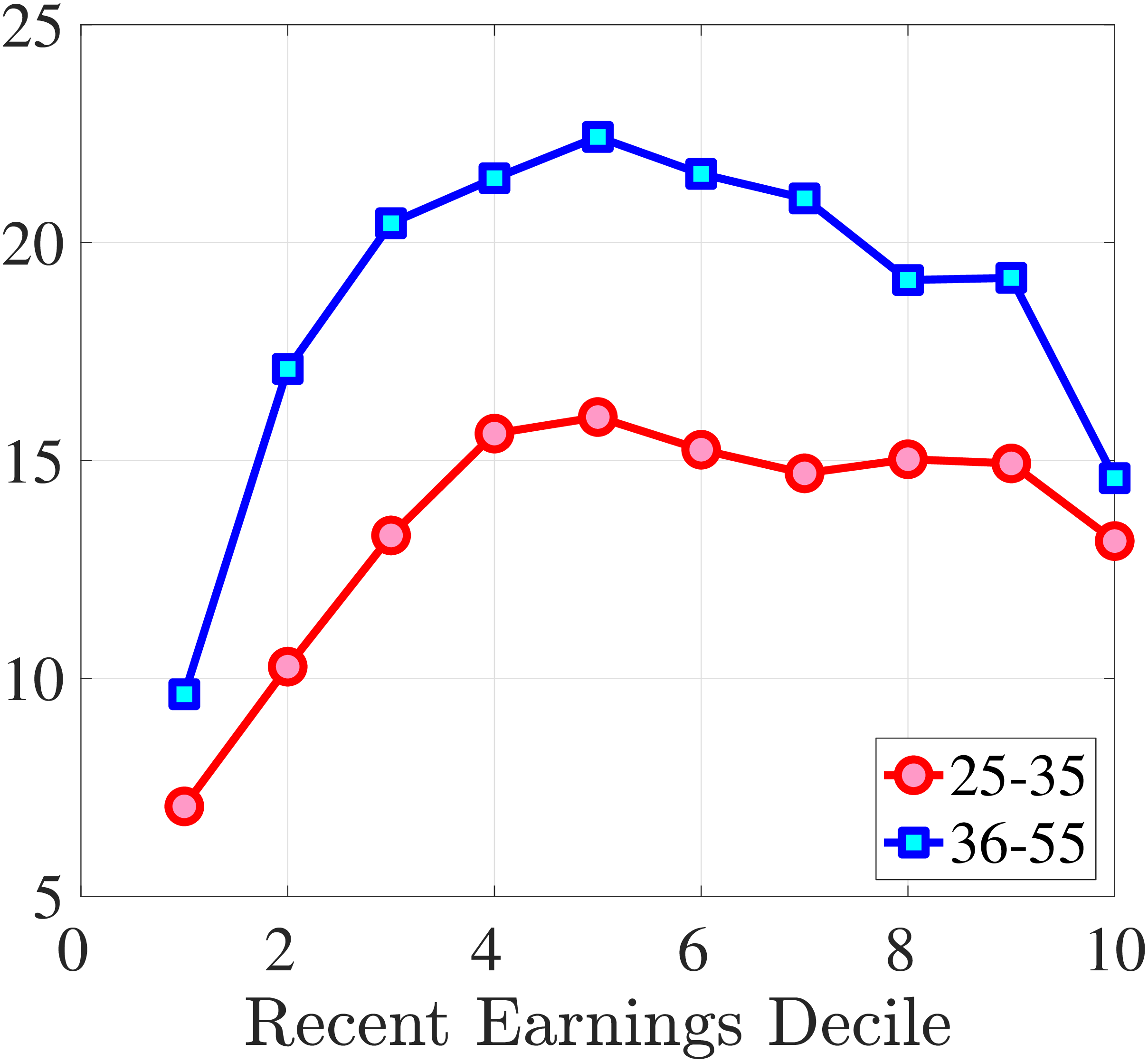(a) Kurtosis of Hourly Wage Changes, $\Delta _{\log}^{5}w_{t}^{i}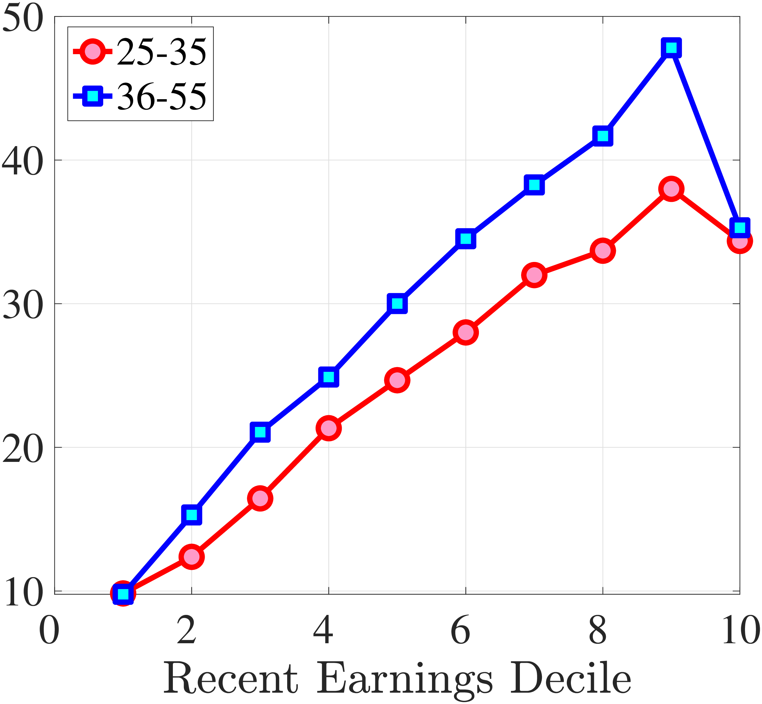$ (b) Kurtosis of Hours Changes, $\Delta _{\log}^{5}h_{t}^{i}$

Figure 11

–

Kurtosis of Five-Year Log Hourly Wage and Hours Growth

Note: The figure plots the kurtosis of five-year wage rate changes (left panel) and hours changes (right panel) by RE decile for young men (red line) and prime-age men (blue line).

Figure: Figure 11 – Kurtosis of Five-Year Log Hourly Wage and Hours Growth

The right panel of Figure 10 decomposes the kurtosis of five-year earnings growth into the contributions from changes in work hours, changes in hourly wages, and the co-kurtosis term using Lemma 1. Up to the median RE, both the wage rate and the hours changes contribute equally to the kurtosis of earnings growth. For higher RE deciles, wage rate growth becomes more important in accounting for the kurtosis of earnings changes, partly because wage changes are larger for these workers. However, the dominant driver of earnings kurtosis tends to be the co-kurtosis terms (except for the top RE groups). Recall that these terms are large if hours and wages tend to undergo large changes concurrently.

Taking Stock. In this section, we have shown that both hours and wage changes are negatively skewed and highly leptokurtic. Both hours and wage rates contribute to the higher-order moments of log earnings growth. However, the main culprit for the large negative skewness and large kurtosis of earnings growth turns out to be the co-skewness and co-kurtosis terms, respectively. Thus, earnings growth is negatively skewed and leptokurtic mainly because of the interaction between hours and wage rate changes. Note that this conclusion may depend on the severity of m.e.. In Appendix A.2, we show that the presence of classical m.e. would bias the estimates of the skewness and kurtosis towrad zero relative to the true skewness and kurtosis of an empirical variable. In this context it is of significant importance that the m.e. in imputed hours is quantitatively small, as argued above.

5.3 Job Stayers and Switchers

Section 4.3 documented that a change of employer is a key event causing large earnings changes. A change of employer can happen either via an unemployment spell or through a direct job-to-job movement. In this section, we study the earnings growth distributions of job stayers and job switchers separately and quantify their role in driving the higher-order moments of earnings growth. To this end, we first identify job stayers and job switchers. We define a job switcher as an individual whose main employer is different between years $t$ and $t+1$, where the main employment is the job that accounts for the largest share of annual earnings. The rest of the population is composed of job stayers.³¹ In other words, a job stayer is a worker whose main employer has remained unchanged for two years in a row, and the job spell is contiguous. This classification of stayer workers is similar to the previous literature (Card et al. (2013)).³²

(a) Variance of $\Delta _{\log}^{1}y_{t}^{i}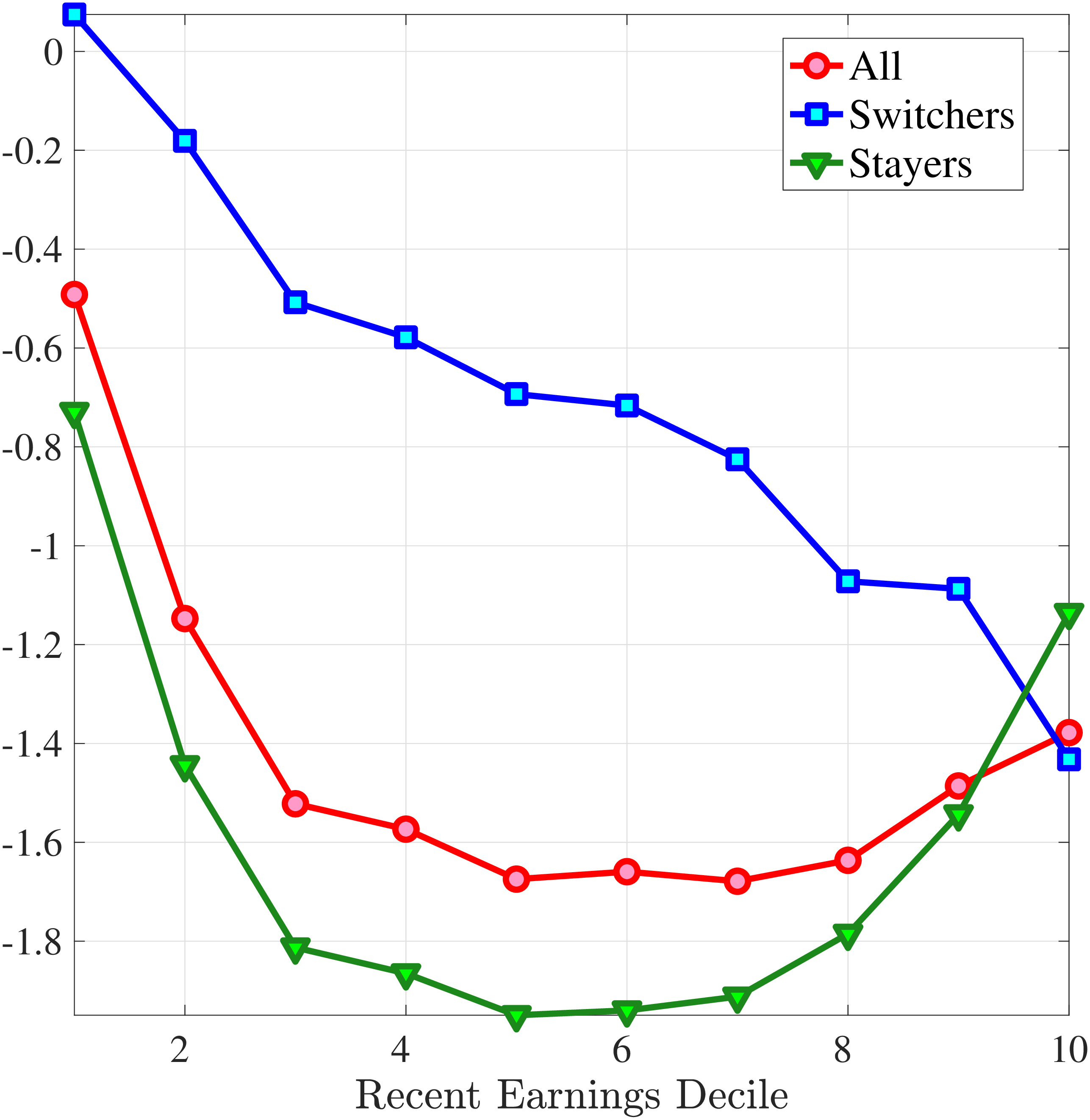$ (b) Skewness of $\Delta _{\log}^{1}y_{t}^{i}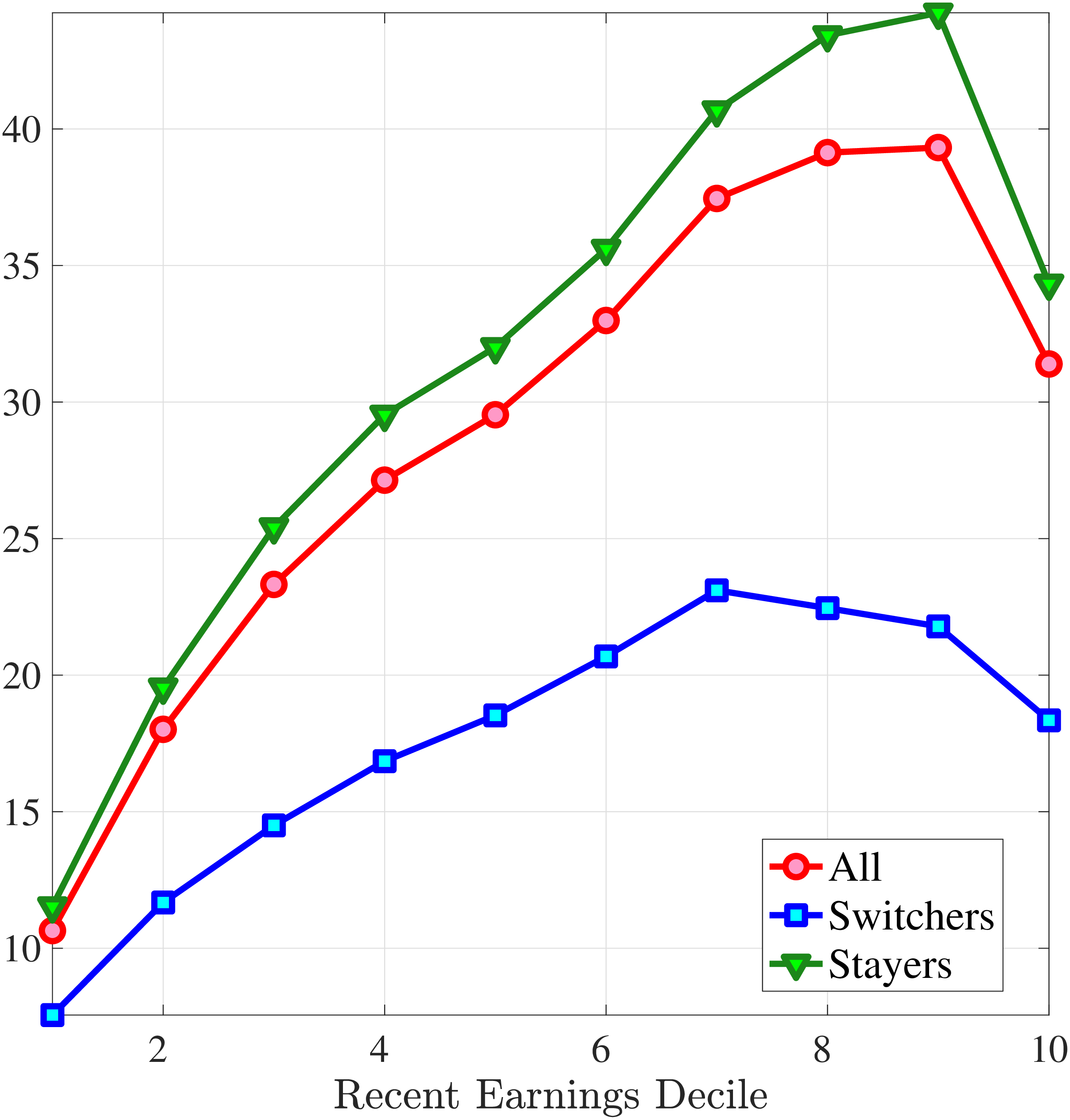$ (c) Kurtosis of $\Delta _{\log}^{1}y_{t}^{i}$

Figure 12

–

Moments of One-Year Log Earnings Growth: Stayers versus Switchers

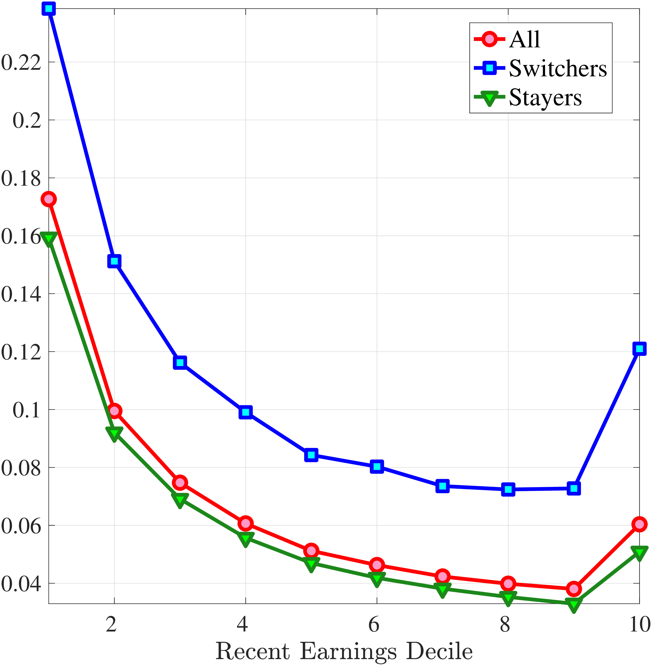
Note: The figure displays the higher-order cross-sectional moments of one-year log earnings growth ($y_{t+1}-y_{t}$) for job switchers (blue line), job stayers (green line), and all prime-age males (red line) for each RE decile.

Figure: Figure 12 – Moments of One-Year Log Earnings Growth: Stayers versus Switchers

Figure 12 shows the cross-sectional moments of one-year earnings growth for stayers and switchers separately. Annual earnings changes for switchers tend to be substantially more dispersed, more symmetric (less left skewed), and significantly less leptokurtic than those for stayers. Figure E.5 in the Appendix confirms that a similar pattern holds for women. The differences between stayers and switchers are qualitatively different from the findings in Guvenen et al. (2019) for the U.S. in that they find that annual earnings growth for males is more symmetric for stayers than it is for switchers. One important contributor to strong negative skewness for stayers in Norway is sickness leave, as workers who receive some sickness benefits have more negative skewness than the stayers who do not experience sickness (details are available upon request). Note that by regulation these workers remain employed by the same firm during their sickness leave.

Role of Stayers and Switchers in Distribution of Earnings Growth

How important are the switchers in driving the nonnormal features of annual earnings growth relative to the stayers? It turns out that the contributions of two mutually exclusive groups, such as job stayers and job switchers, to the cross-sectional skewness and kurtosis of earnings changes can be decomposed using two simple formulas that we state in the following lemma.

Lemma 2. Let the sample $S$ be split into two mutually exclusive groups, $S=S_{1}\cup S_{2}$ and $S_{1}\cap S_{2}=\emptyset$. Skewness can then be decomposed into $S_{1}$ and $S_{2}$ components,

\[ \begin{aligned} \text{skew}\left (y\right) &= \underset{\text{skewness due to }S_{1}}{\underbrace{\frac{1}{\left (std\left (y\right)\right)^{3}}\int _{\left \{i\in S_{1}\right \}}\left (y_{i}-E\left (y\right)\right)^{3}dF\left (y\right)}}+\underset{\text{skewness due to }S_{2}}{\underbrace{\frac{1}{\left (std\left (y\right)\right)^{3}}\int _{\left \{i\in S_{2}\right \}}\left (y_{i}-E\left (y\right)\right)^{3}dF\left (y\right)}}. \end{aligned} \]

Kurtosis can be decomposed into components stemming from $S_{1}$ and $S_{2}$,

\[ \begin{aligned} \text{kurt}\left (y\right) &= \underset{\text{kurtosis due to }S_{1}}{\underbrace{\frac{1}{\left (std\left (y\right)\right)^{4}}\int _{\left \{i\in S_{1}\right \}}\left (y_{i}-E\left (y\right)\right)^{4}dF\left (y\right)}}+\underset{\text{kurtosis due to }S_{2}}{\underbrace{\frac{1}{\left (std\left (y\right)\right)^{4}}\int _{\left \{i\in S_{2}\right \}}\left (y_{i}-E\left (y\right)\right)^{4}dF\left (y\right)}}. \end{aligned} \]

In Figure 13, we use Lemma 2 to decompose the population skewness and kurtosis of one-year earnings growth into the contribution of job stayers and the contribution of job switchers. The negative skewness and high kurtosis of earnings growth are overwhelmingly driven by job stayers. The reason is twofold. First, the skewness is more negative and the kurtosis larger for stayers than for switchers. Second, there are very few switchers relative to the number of stayers. The expressions in Lemma 2 show that the contributions from each of the mutually exclusive subsets to the third and fourth centralized moments of their union are proportional to their population size.

Skewness

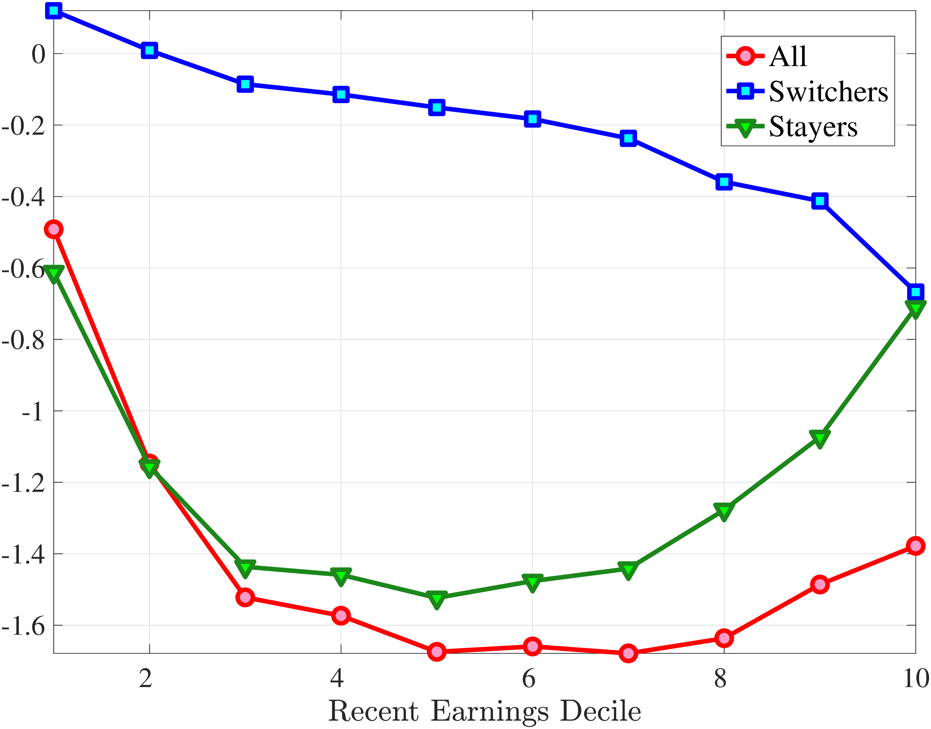
Kurtosis

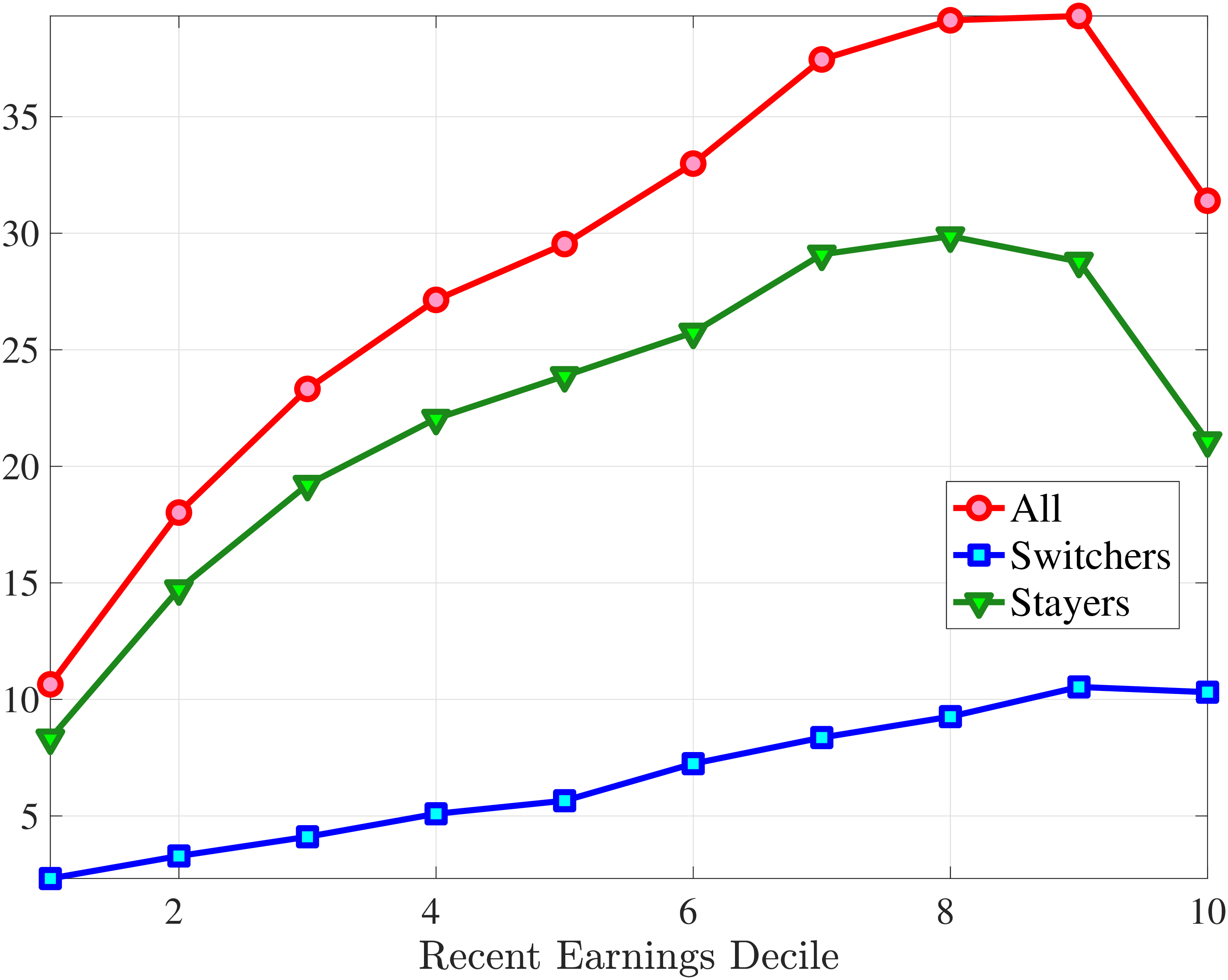
Figure 13

–

Moment Decomposition of Earnings Growth: Stayers vs. Switchers

Note: The figure displays the contributions of job switchers (blue line) and job stayers (green line) to the population skewness and kurtosis of one-year earnings growth for prime-age males (red line) for each RE decile.

Figure: Figure 13 – Moment Decomposition of Earnings Growth: Stayers vs. Switchers

5.4 Cross-Sectional Moments of Household Labor and Disposable Income Growth

Thus far, we have focused on the distribution of fluctuations in male labor earnings. However, for many economic questions, household disposable income after taxes and transfers, rather than individual male or female labor income before taxes, is more important. For example, for consumption and risk sharing, the relevant risk is that for disposable income. In this section, we investigate the moments of shocks to household labor income and household disposable income for married couples. Since these calculations do not require the imputation of hours worked, we no longer need data on register hours. This allows us to extend the sample to include the years $t\in [1998,2002]$. We also do not drop individuals with less than 200 hours worked per year but still require them to have earnings above a minimum income threshold, $Y_{min,t}.$ We report two measures of disposable income. We define “household disposable income” as labor and capital income plus transfers minus taxes. We also study “household disposable labor income,” which we define as household disposable income net of capital income and capital taxes (which take the form of a 28% flat tax on capital income). Namely, disposable labor income is labor income after taxes and transfers. Transfers include unemployment benefits, sickness benefits, paid parental leave, remuneration for participation in various government activity programs, disability benefits, public pensions, and other social welfare payments.³³

(a) Variance of $\Delta _{\log}^{5}z_{t}^{i}$

$(a) Variance of $\Delta _{\log}^{5}z_{t}^{i}$$

(b) Skewness of $\Delta _{\log}^{5}z_{t}^{i}$

$(b) Skewness of $\Delta _{\log}^{5}z_{t}^{i}$$

$(c) Kurtosis of $\Delta _{\log}^{5}z_{t}^{i}$$

Figure 14 – Moments of 5-Year Household Earnings and Disp. Income Growth, Ages 36-55

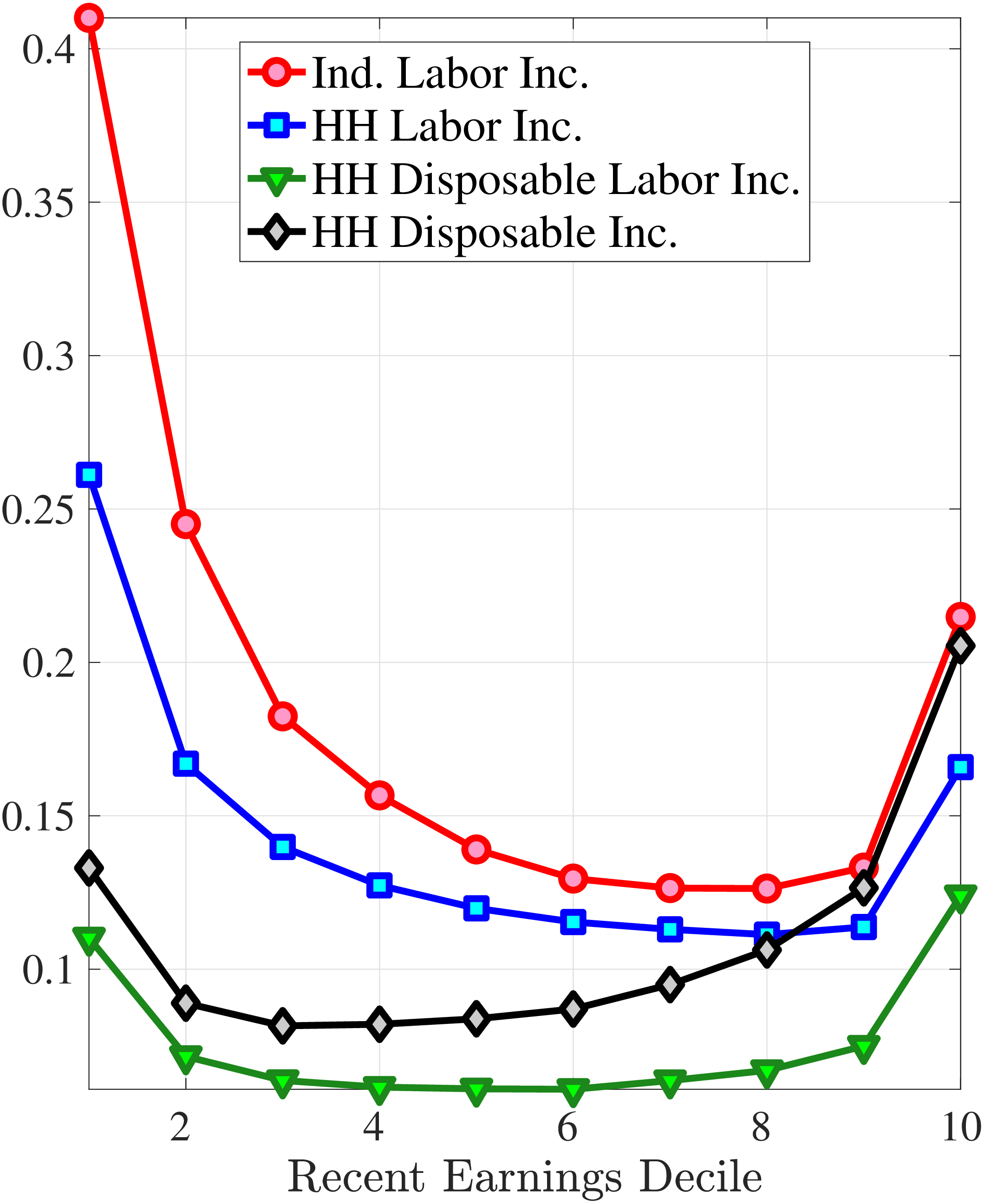
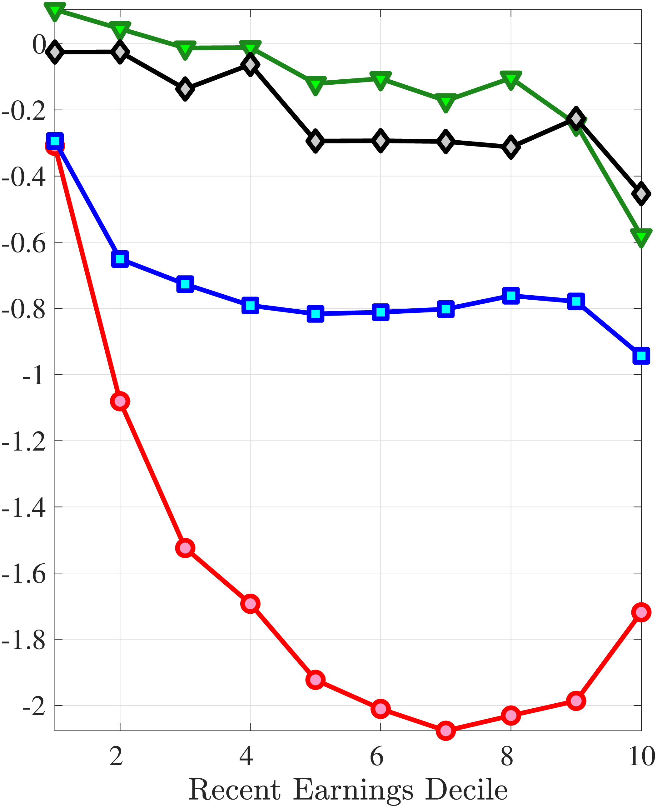
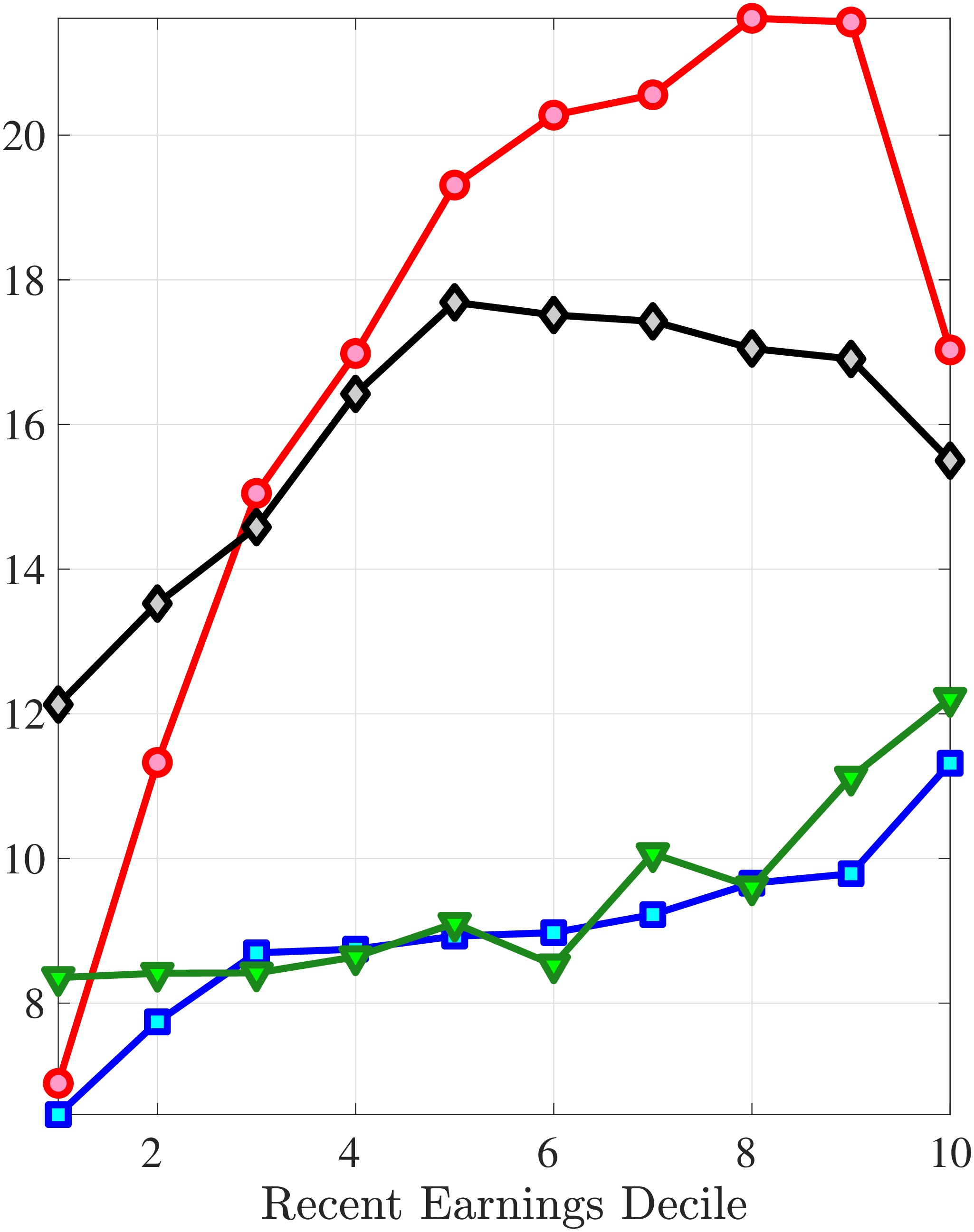
Note: The figure displays the higher-order cross-sectional moments of five-year log earnings changes (red line), log household earnings changes (blue line), log disposable labor income changes (green line), and log disposable income changes (black line) for prime-age males, plotted for each decile of RE. Disposable labor income is defined as disposable income net of after-tax capital income. The sample comprises married and cohabiting men and their households.

(a) Variance of $\Delta _{\log}^{5}z_{t}^{i}$

$(a) Variance of $\Delta _{\log}^{5}z_{t}^{i}$$

(b) Skewness of $\Delta _{\log}^{5}z_{t}^{i}$

$(b) Skewness of $\Delta _{\log}^{5}z_{t}^{i}$$

$(c) Kurtosis of $\Delta _{\log}^{5}z_{t}^{i}$$

Figure 15 – Moments of 5-Year Household Earnings and Disp. Income Growth, Ages 25-35

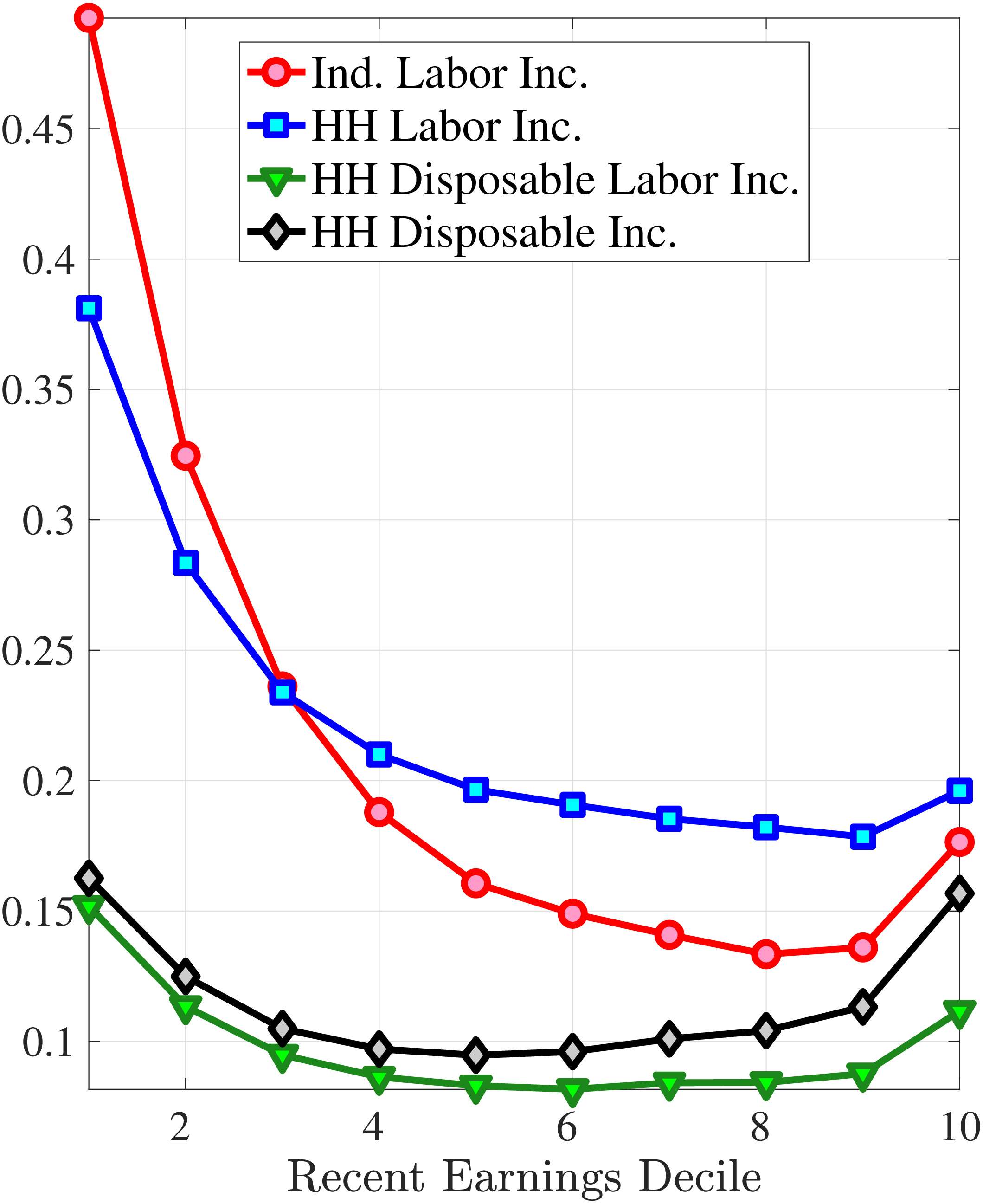
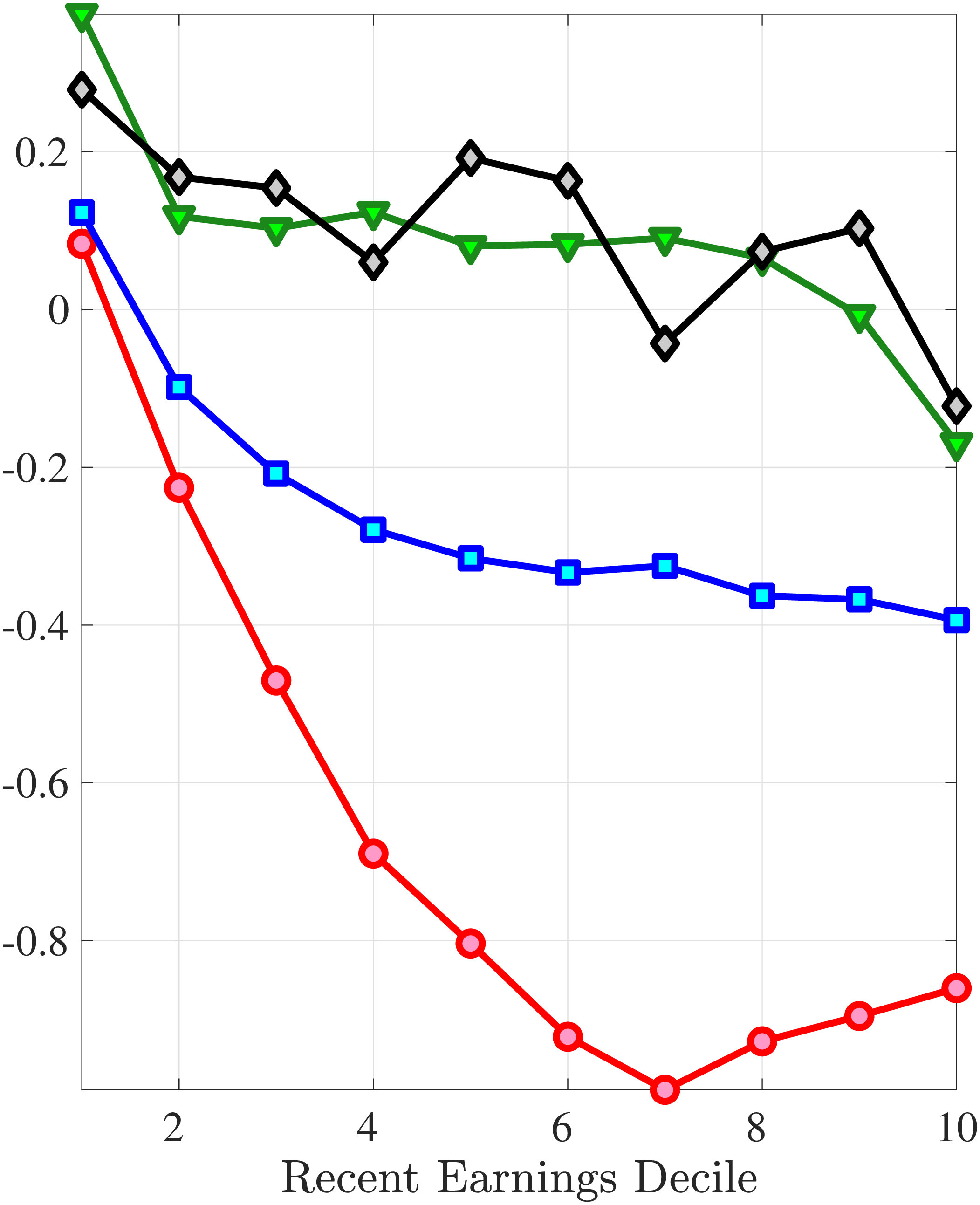
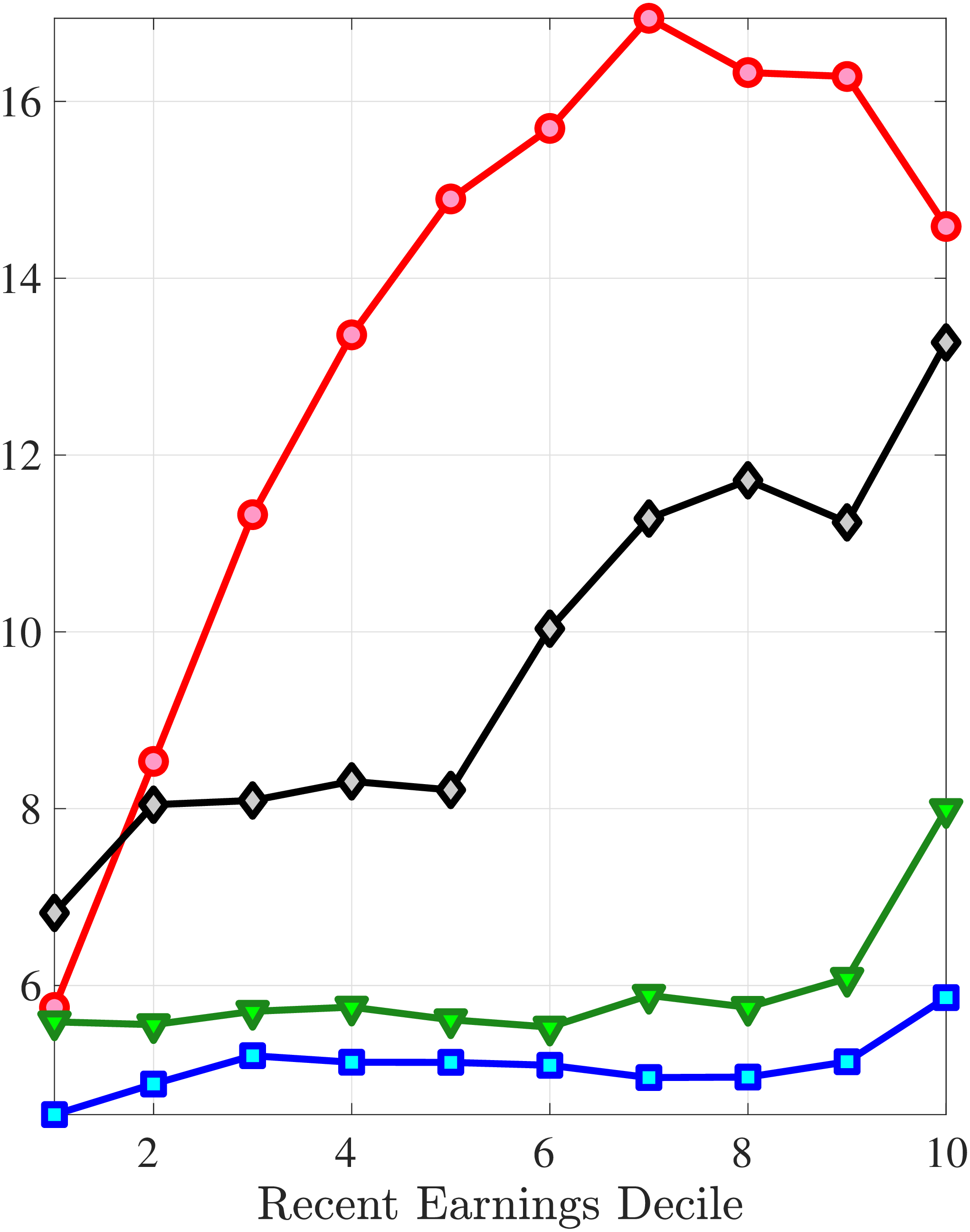
Note: The figure displays the higher-order cross-sectional moments of five-year log earnings changes (red line), log household earnings changes (blue line), and log disposable labor income changes (green line), and log disposable income changes (black line) for young males, plotted for each decile of RE. Disposable labor income is defined as disposable income net of after-tax capital income. The sample comprises married and cohabiting men and their households.

In Figures 14a and 15a, we plot the variance of five-year income growth for individual earnings, household earnings, and household disposable income for males living as part of a couple (married and cohabiting men) by recent earnings decile for prime-age and young workers, respectively. Figures B.19 and B.20 in the Appendix report the same moments for one-year income growth measures. Consider first the difference between the variance of changes in individual male earnings (red line in Figures 14a and 15a) and changes in household earnings (blue line). For older workers, the variance of changes is somewhat lower for household earnings than for individual earnings, whereas for younger workers, the variance is actually larger for household earnings than for individual male earnings, except for the poorest workers. This suggests that older couples face slightly lower before-tax earnings fluctuations relative to individual men, whereas household earnings are more volatile than male earnings for younger couples. This finding might seem surprising in that household earnings change substantially less than male earnings in response to a change in male earnings. However, female earnings are also subject to large changes, and household earnings incorporate shocks to the earnings of both spouses.

Consider next the variance of changes in disposable household labor income (green line in Figures 14a and 15a). These variances are reduced by more than 50% relative to the variance of changes in individual and household labor earnings. This suggests that taxes and transfers provide substantial insurance against individual earnings risk and that this holds true across the income distribution. The reduction is somewhat larger for low-income men. For this group, the main culprit for reducing the variance of changes is the generous Norwegian welfare benefits (unemployment insurance, disability insurance, social aid, and cash benefits to families with children).³⁴ Our findings are in line with Blundell et al. (2014), who study how risk changes over the life cycle using the same administrative data from Norway. They estimate models with transitory and persistent income shocks and show that the variances of both transitory and persistent shocks fall substantially when going from individual earnings to household disposable labor income.³⁵ Finally, we add in capital income and consider the variance of changes in disposable household income (black lines in Figures 14a and 15a). This increases the variance of income growth relative to the growth in disposable labor income. Thus, capital income tends to increase the variance of disposable income growth. This increase is larger for households above the median RE.

To our knowledge, we are the first to document how the moments of income growth rates—including the variance—change when going from individual labor income to household labor income and, finally, to our two notions of disposable income growth. Heathcote et al. (2010a) document how the variance of disposable income (in levels) changes when going through a similar sequence of income concepts.

With respect to skewness, Figures 14b and 15b plot the skewness for five-year income growth for individual male earnings, household earnings, household disposable labor income, and household disposable income by RE decile. As can be seen from the figures, changes in household earnings are substantially less negatively skewed than male earnings changes. This finding is in line with what Pruitt and Turner (2018) found for the U.S. Note that this reduction in left skewness is not due to behavioral changes in spousal earnings. In Figure D.7 in the Appendix, we show that spousal earnings are remarkably unresponsive to changes in male earnings, for both positive and negative changes. Thus, we interpret the reduction in negative skewness as a mechanical second-earner effect, namely, that a change in male earnings has a smaller effect on household earnings simply because household earnings is the sum of earnings for the two spouses.

Figures 14b and 15b reveal that the effect of going to disposable income is even starker: five-year changes in disposable income have close to zero skewness. Moreover, Figures B.19 and B.20 in the Appendix show that the skewness of one-year changes is strongly positive for many RE-groups, for both changes in household disposable income and changes in household disposable labor income. In conclusion, both the tax and transfer system and spousal income contribute to removing the negative skewness of wage earnings growth, making five-year household disposable income growth approximately symmetric and one-year disposable income growth right skewed.

In Figures 14c and 15c, we plot the kurtosis for five-year income growth for the four notions of income (individual earnings, household earnings, and so on) for males living as part of a couple by RE decile. The kurtosis of household earnings growth is significantly lower than for individual labor income. For men above the median, the kurtosis is reduced by around two-thirds when going from individual labor income to household labor income. Finally, as one might expect, the kurtosis of disposable income growth is substantially higher than for household labor income growth, reflecting that capital income in the form of dividends and capital gains tends to see frequent small changes and infrequent large changes, inducing higher kurtosis.

Overall, these results show that the higher-order moments for disposable income growth and, to a smaller extent, household earnings growth differ sharply from those of male earnings growth. In particular, disposable income is essentially symmetrically distributed. Moreover, changes in disposable income have substantially lower variance than changes in male earnings. However, the kurtosis for disposable income growth is comparable to the kurtosis of individual earnings growth: slightly larger for poorer households and lower for the richest ones.

6 Conclusion

This paper studies the drivers behind two important deviations from standard linear and symmetric models of labor income risk, namely, asymmetric mean reversion of earnings changes—large negative changes are less persistent than positive changes—and more negative skewness and higher kurtosis relative to a Gaussian distribution. Using Norwegian administrative register data and labor survey data, we decompose earnings into hours and hourly wages and examine the extent to which the nonlinearities in mean reversion and non-Gaussian higher-order moments are caused by hours or hourly wages.

We find that the nonlinear mean reversion in earnings is mainly driven by the dynamics of hours worked, whereas wage rate dynamics play a less important role. Indeed, hours dynamics are very nonlinear: negative changes are relatively transient, whereas positive changes are close to permanent. In contrast, wage rate dynamics are close to being linear, with both positive and negative changes being highly persistent. These findings are based on following groups of people who experience a similar initial change, and this approach captures the effects that work through both the intensive and extensive margins of labor supply. The fact that declines in hours worked are transitory while wage rate changes are more persistent offers an immediate implication for government insurance policies against falls in labor income: since it is more difficult for households to self-insure against persistent shocks than against transitory shocks, the welfare state should aim at providing long-term insurance against wage rate fluctuations rather than insuring fluctuations in hours. Wage compression would be one example of an institution that provides insurance against wage rate shocks. Such compression might take place through bargaining between labor unions and employers or through wage-moderation norms. Wage compression could also be achieved through government policies. A minimum wage mandate is an example of such a policy. Another example would be to allow progressive taxation directly on hourly wage rates, implying that the progressivity on wage rates would be higher than the progressivity on labor earnings. Finally, consider the case of standard unemployment insurance. Such a program provides assistance only during times of unemployment and ends once the worker returns to employment. Thus, while unemployment insurance might provide adequate insurance against fluctuations in hours, it fails to provide long-term insurance against wage rate fluctuations. We leave it to future work to further explore the optimality and feasibility of the tax progressivity of hourly wage rates versus labor earnings.

As for higher-order moments, we document that, first, individual labor income dynamics in Norway are remarkably similar to their counterparts in U.S. data, in terms of both nonlinear persistence and higher-order moments. Second, we find that both wage rates and hours worked contribute to the negative skewness and high kurtosis of individual earnings changes. However, the interaction between hours and wages—captured by the co-skewness and co-kurtosis terms—is quantitatively most important. Finally, the Norwegian register data allow us to identify individuals in households. We show that the deviations from normality are mitigated for household earnings and disposable household income compared to male labor earnings. In fact, changes in disposable household income are almost symmetric, which also suggests that one should not expect to see negative skewness in consumption changes.

While our study is based on data from Norway, we believe the findings also have general validity for other countries, including the U.S. The fact that earnings dynamics for Norway and the U.S. are quantitatively and qualitatively similar despite the differences in labor market institutions across these countries suggests that Norwegian and U.S. earnings dynamics may be driven by similar economic mechanisms.

References

Abowd, J. M. and Card, D. (1989). On the covariance structure of earnings and hours changes. Econometrica, 57 (2), 411–45.

Altonji, J. G. (1986). Intertemporal substitution in labor supply: Evidence from micro data. Journal of Political Economy, 94 (3), S176–S215.

Arellano, M., Blundell, R. and Bonhomme, S. (2017). Earnings and consumption dynamics: a nonlinear panel data framework. Econometrica, 85 (3), 693–734.

Attanasio, O. and Davis, S. J. (1996). Relative wage movements and the distribution of consumption. Journal of Political Economy, 104 (6), 1227–62.

Bick, A., Blandin, A. and Rogerson, R. (2022). Hours and wages. Quarterly Journal of Economics.

Blundell, R., Graber, M. and Mogstad, M. (2014). Labor income dynamics and the insurance from taxes, transfers, and the family. Journal of Public Economics.

—, Pistaferri, L. and Preston, I. (2008). Consumption inequality and partial insurance. American Economic Review, 98 (5), 1887–1921.

— and Preston, I. (1998). Consumption inequality and income uncertainty. The Quarterly Journal of Economics, 113 (2), 603–640.

Busch, C., Domeij, D., Guvenen, F. and Madera, R. (2018). Asymmetric business-cycle risk and social insurance. Woking paper.

Card, D., Heining, J. and Kline, P. (2013). Workplace Heterogeneity and the Rise of West German Wage Inequality. The Quarterly Journal of Economics, 128 (3), 967–1015.

Chakraborty, I., Holter, H. A. and Stepanchuk, S. (2015). Marriage stability, taxation and aggregate labor supply in the u.s. vs. europe. Journal of Monetary Economics, 72, 1–20.

Cochrane, J. H. (1991). A simple test of consumption insurance. Journal of Political Economy, 99 (5), 957–76.

Conesa, J. C., Kitao, S. and Krueger, D. (2009). Taxing capital? not a bad idea after all! American Economic Review, 99 (1), 25–48.

Cutler, D. M. and Katz, L. F. (1992). Rising inequality? changes in the distribution of income and consumption in the 1980's. American Economic Review, 82 (2), 546–51.

De Nardi, M., Fella, G., Knoef, M., Ooijen, R. V. and Pardo, G. P. (2021). Family and government insurance: Wage, earnings, and income risks in the netherlands and the u.s. Journal of Public Economics, 193.

Deaton, A. and Paxson, C. (1994). Intertemporal choice and inequality. Journal of Political Economy, 102 (3), 437–67.

Guvenen, F., Karahan, F. and Ozkan, S. (2018). Inequality over the Life Cycle in the Presence of Higher-Order Risk. Working paper, University of Minnesota.

—, —, — and Song, J. (2019). What Do Data on Millions of U.S. Workers Say About Labor Income Risk? Working Paper 20913, National Bureau of Economic Research.

—, Ozkan, S. and Song, J. (2014). The Nature of Countercyclical Income Risk. Journal of Political Economy, 122 (3), 621–660.

Hastie, T., Tibshirani, R., Friedman, J. H. and Friedman, J. H. (2009). The elements of statistical learning: data mining, inference, and prediction, vol. 2. Springer.

Heathcote, J., Perri, F. and Violante, G. L. (2010a). Unequal we stand: An empirical analysis of economic inequality in the united states, 1967-2006. Review of Economic Dynamics, 13 (1), 15–51.

—, Storesletten, K. and Violante, G. L. (2009). Quantitative macroeconomics with heterogeneous households. Annual Review of Economics, 1, 319–354.

—, — and — (2010b). The macroeconomic implications of rising wage inequality in the united states. Journal of Political Economy, 118 (4), 681–722.

—, — and — (2014). Consumption and labor supply with partial insurance: An analytical framework. American Economic Review.

Hubmer, J. (2018). The job ladder and its implications for earnings risk. Review of Economic Dynamics, 29, 172–194.

Huttunen, K., Moen, J. and Salvanes, K. G. (2011). How destructive is creative destruction? effects of job loss on job mobility, withdrawal and income. Journal of the European Economic Association, 9 (5), 840–870.

Jacobson, L. S., LaLonde, R. J. and Sullivan, D. G. (1993). Earnings losses of displaced workers. American Economic Review, 83 (4), 685–709.

Jarosch, G. (2021). Searching for Job Security and the Consequences of Job Loss. Working paper, Princeton University.

Karahan, F., Ozkan, S. and Song, J. (2019). Anatomy of lifetime earnings inequality: Heterogeneity in job ladder risk vs. human capital. FRB of New York Staff Report, (908).

Krueger, D. and Perri, F. (2005). Does income inequality lead to consumption inequality? evidence and theory. Review of Economic Studies, 73 (1), 163–193.

Krusell, P., Mukoyama, T., Rogerson, R. and Sahin, A. (2011). A three state model of worker flows in general equilibrium. Journal of Economic Theory, 146 (3), 1107–1133.

Lillard, L. A. and Weiss, Y. (1979). Components of variation in panel earnings data: American scientists 1960-70. Econometrica, 47 (2), 437–454.

— and Willis, R. J. (1978). Dynamic aspects of earnings mobility. Econometrica, 46 (5), 985–1012.

Loh, W.-Y. (2011). Classification and regression trees. Wiley interdisciplinary reviews: data mining and knowledge discovery, 1 (1), 14–23.

MaCurdy, T. E. (1981). An empirical model of labor supply in a life-cycle setting. Journal of political Economy, 89 (6), 1059–1085.

— (1982). The Use of Time Series Process to Model the Error Structure of Earnings in a Longitudinal Data Analysis. Journal of Econometrics, 18, 83–114.

Parker, J. A. and Vissing-Jorgensen, A. (2010). The increase in income cyclicality of high-income households and its relation to the rise in top income shares. Brookings Papers on Economic Activity, 41 (2), 1–70.

Pruitt, S. and Turner, N. (2018). The nature of household labor income risk. Woking paper.

Quinlan, J. R. (1992). Learning with continuous classes. In Proceedings Australian Joint Conference on Artificial Intelligence, World Scientific, pp. 343–348.

Von Wachter, T., Song, J. and Manchester, J. (2009). Long-Term Earnings Losses due to Mass Layoffs During the 1982 Recession: An Analysis Using U.S. Administrative Data from 1974 to 2004. Tech. rep., Columbia University.

Appendices

7 Derivations and Imputation of Hours

7.1 Proof of Lemma 1

The formula for skewness is skew(x)=E(x-E(x))^{3}. Consider the skewness of a sum of stochastic variables:

\[ \begin{aligned} \text{skew}\left (x+y\right) &= \frac{1}{\left (std\left (x+y\right)\right)^{3}}E\left (x+y-E\left (x+y\right)\right)^{3}\\ &= \frac{1}{\left (std\left (x+y\right)\right)^{3}}E\left \{\left [x-E\left (x\right)\right]^{3}+\left [y-E\left (y\right)\right]^{3}+3\left [x-E\left (x\right)\right]^{2}\left [y-E\left (y\right)\right]+3\left [x-E\left (x\right)\right]\left [y-E\left (y\right)\right]^{2}\right \}\\ &= \left (\frac{std\left (x\right)}{std\left (x+y\right)}\right)^{3}\cdot \text{skew}\left (x\right)+\left (\frac{std\left (y\right)}{std\left (x+y\right)}\right)^{3}\cdot \text{skew}\left (y\right)\\ & +\frac{3}{\left (std\left (x+y\right)\right)^{3}}\left (cov\left (x^{2},y\right)+cov\left (x,y^{2}\right)-2\left (E\{y\}+E\{x\}\right)\cdot cov\left (x,y\right)\right), \end{aligned} \]

where the second to last equality is due to

\[ \begin{aligned} & E\left (\left (x-E\{x\}\right)^{2}\left (y-E\{y\}\right)\right)\\ &= E\left (x^{2}y\right)-E\{y\}E\left (x^{2}\right)-2E\{x\}\left (E\left (xy\right)-E\{y\}E\{x\}\right)+E\left (E\{x\}^{2}\left (y-E\{y\}\right)\right)\\ &= cov\left (x^{2},y\right)-2E\{x\}\cdot cov\left (x,y\right). \end{aligned} \]

The formula for the fourth central moment, kurtosis, is \[ \text{kurt}\left (x\right)=\frac{1}{\left (std\left (x\right)\right)^{4}}E\left (x-E\left (x\right)\right)^{4}. \] Consider now the kurtosis of a sum of stochastic variables and keeping in mind that: $\left (x+y\right)^{4}=x^{4}+4x^{3}y+6x^{2}y^{2}+4xy^{3}+y^{4}$ we have:

\[ \begin{aligned} \text{kurt}\left (x+y\right) &= \frac{1}{\left (std\left (x+y\right)\right)^{4}}E\left (x+y-E\left (x+y\right)\right)^{4}\\ &= \frac{1}{\left (var\left (x+y\right)\right)^{2}}E\left \{\left [x-E\left (x\right)\right]^{4}+\left [y-E\left (y\right)\right]^{4}+4\left [x-E\left (x\right)\right]^{3}\left [y-E\left (y\right)\right]+4\left [x-E\left (x\right)\right]\left [y-E\left (y\right)\right]^{3}\right \}\\ & +\frac{1}{\left (var\left (x+y\right)\right)^{2}}E\left \{6\left [x-E\left (x\right)\right]^{2}\left [y-E\left (y\right)\right]^{2}\right \}\\ &= \left (\frac{var\left (x\right)}{var\left (x+y\right)}\right)^{2}\text{kurt}\left (x\right)+\left (\frac{var\left (y\right)}{var\left (x+y\right)}\right)^{2}\text{kurt}\left (y\right)+X, \end{aligned} \]

where $X$ captures a set of co-variance and co-skewness terms, X^{3}} +2E{^{3}} +3E{^{2}^{2}} ].

7.2 Higher-Order Moments with Classical Measurement Error in Hours

This section addresses how classical m.e. in hours would affect the estimates of higher- order moments. Even though our imputation methodology does a good job at predicting annual hours worked, some m.e. may still be inevitable. We now analyze how our estimates of the higher-order moments of hours and wage changes would be biased because of m.e.. Consider a simple model of m.e., $\hat{z}=z+\hat{\varepsilon}$, where $\hat{z}$ denotes the measure of a variable observed in the data, $\hat{\varepsilon}$ denotes m.e., and $z$ is the true value of the variable. The following lemma establishes how m.e. influences the moments.

Lemma 3.

Assume that m.e. $\hat{\varepsilon}$ is independent of the true variable $z$. Then, the estimates for the skewness and kurtosis of the measured variable $\hat{z}$ are given by

\[ \begin{aligned} skew\left (\hat{z}\right)= & \left (\frac{var\left (z\right)}{var\left (z\right)+var\left (\hat{\varepsilon}\right)}\right)^{\frac{3}{2}} & skew(z)+\left (\frac{var\left (\hat{\varepsilon}\right)}{var\left (z\right)+var\left (\hat{\varepsilon}\right)}\right)^{\frac{3}{2}}skew\left (\hat{\varepsilon}\right)\\ kurt\left (\hat{z}\right)= & \left (\frac{var\left (z\right)}{var\left (z\right)+var\left (\hat{\varepsilon}\right)}\right)^{2} & kurt(z)+\left (\frac{var\left (\hat{\varepsilon}\right)}{var\left (z\right)+var\left (\hat{\varepsilon}\right)}\right)^{2}kurt\left (\hat{\varepsilon}\right)+\frac{6\cdot var\left (\hat{\varepsilon}\right)\cdot var\left (z\right)}{\left (var\left (z\right)+var\left (\hat{\varepsilon}\right)\right)^{2}}, \end{aligned} \]

where $skew$ and $kurt$ are the third and fourth centralized moments for skewness and excess kurtosis (i.e., fourth centralized moment minus 3), respectively.

Proof. See Sections A.2.1 and A.2.2 below. □

Suppose that m.e. is classical (i.e., that it has a symmetric distribution with $skew\left (\hat{\varepsilon}\right)=0$ and $kurt\left (\hat{\varepsilon}\right)>0$). In this case, the lemma shows that the skewness of the measured hours and wage growth would be biased toward zero relative to the true skewness (see Section A.2). For kurtosis, the bias could go either way. Thus, we believe that our findings in this section are upper bounds for the true skewness of hours and wage changes.

Let $z$ and $\hat{z}$ denote the true value of the random variable z and the measured value of z, respectively. Assume that the m.e. in z is classical, $\hat{z}=z+\hat{\varepsilon}$. This m.e. is then inherited in the empirical moments, for example, in variance, $var\left (\hat{z}\right)=var\left (z\right)+var\left (\hat{\varepsilon}\right)$.

7.2.1 Skewness

Consider now the third moment (skewness):

\[ \begin{aligned} \text{skew}\left (\hat{z}\right) &= \frac{1}{\left (\sigma \left (\hat{z}\right)\right)^{3}}E\left (\hat{z}-E\left (\hat{z}\right)\right)^{3}=\frac{1}{\left (var\left (z\right)+var\left (\hat{\varepsilon}\right)\right)^{\frac{3}{2}}}E\left (z+\hat{\varepsilon}-E\left (z\right)\right)^{3}\\ &= \left (\frac{var\left (z\right)}{var\left (z\right)+var\left (\hat{\varepsilon}\right)}\right)^{\frac{3}{2}}\cdot S\left (z\right)+\left (\frac{var\left (\hat{\varepsilon}\right)}{var\left (z\right)+var\left (\hat{\varepsilon}\right)}\right)^{\frac{3}{2}}\cdot S\left (\hat{\varepsilon}\right). \end{aligned} \]

Thus, the measured skewness is a weighted sum of the true skewness of $z$, ($S\left (z\right)$), and the skewness of the m.e., ($S\left (\hat{\varepsilon}\right)$), where the weights do not sum to unity. It follows that the true skewness of $z$ is given by

\[ \begin{aligned} S\left (z\right) &= \left (\frac{var\left (z\right)+var\left (\hat{\varepsilon}\right)}{var\left (z\right)}\right)^{\frac{3}{2}}S\left (\hat{z}\right)-\left (\frac{var\left (\hat{\varepsilon}\right)}{var\left (z\right)}\right)^{\frac{3}{2}}\cdot S\left (\hat{\varepsilon}\right). \end{aligned} \]

Thus, if we assume that the m.e. is normally distributed, then the measured skewness is biased toward zero relative to the true skewness:

\[ \begin{aligned} S\left (z\right) &= \left (\frac{var\left (z\right)+var\left (\hat{\varepsilon}\right)}{var\left (z\right)}\right)^{\frac{3}{2}}S\left (\hat{z}\right). \end{aligned} \]

7.2.2 Kurtosis

Finally, consider the fourth moment: (z)E(z-E(z))^{4}. This implies that the measured kurtosis of $z$ can be expressed as

\[ \begin{aligned} \text{kurt}\left (\hat{z}\right) &= \frac{1}{\left (\sigma \left (\hat{z}\right)\right)^{4}}E\left (\hat{z}-E\left (\hat{z}\right)\right)^{4}=\frac{1}{\left (var\left (z\right)+var\left (\hat{\varepsilon}\right)\right)^{2}}E\left (z+\hat{\varepsilon}-E\left (z\right)\right)^{4}\\ &= \left (\frac{var\left (z\right)}{var\left (z\right)+var\left (\hat{\varepsilon}\right)}\right)^{2}\cdot \text{kurt}\left (z\right)+\left (\frac{var\left (\hat{\varepsilon}\right)}{var\left (z\right)+var\left (\hat{\varepsilon}\right)}\right)^{2}\cdot \text{kurt}\left (\hat{\varepsilon}\right)+\frac{6\cdot var\left (\hat{\varepsilon}\right)\cdot var\left (z\right)}{\left (var\left (z\right)+var\left (\hat{\varepsilon}\right)\right)^{2}}. \end{aligned} \]

It then follows that the true kurtosis of $z$ is given by

\[ \begin{aligned} \text{kurt}\left (z\right) &= \left (1+\frac{var\left (\hat{\varepsilon}\right)}{var\left (z\right)}\right)^{2}\text{kurt}\left (\hat{h}\right)-\left (\frac{var\left (\hat{\varepsilon}\right)}{var\left (z\right)}\right)^{2}\cdot \text{kurt}\left (\hat{\varepsilon}\right)-6\cdot \frac{var\left (\hat{\varepsilon}\right)}{var\left (z\right)} \end{aligned} \]

The true excess kurtosis of $z$ is then given by

\[ \begin{aligned} \text{excess kurt}\left (z\right) &= \left (1+\frac{var\left (\hat{\varepsilon}\right)}{var\left (z\right)}\right)^{2}\text{excess kurt}\left (\hat{z}\right)-\left (\frac{var\left (\hat{\varepsilon}\right)}{var\left (z\right)}\right)^{2}\cdot \text{excess kurt}\left (\hat{\varepsilon}\right). \end{aligned} \]

If we assume that m.e. is normally distributed, the measured excess kurtosis is biased toward zero relative to the true excess kurtosis:

\[ \begin{aligned} \text{excess kurt}\left (z\right) &= \left (1+\frac{var\left (\hat{\varepsilon}\right)}{var\left (z\right)}\right)^{2}\text{excess kurt}\left (\hat{z}\right). \end{aligned} \]

Imputing Hours in the Register Data

7.3 Labor Force Survey (AKU)

The Norwegian Labor Force Survey (AKU) is a representative survey of all persons age 15-74 years and registered as residents in Norway. Before 2006, the age group was 16-74 years, defined as the age at the end of the year. From 2006 on, age is defined as years of age at the reference times for the survey. At the same time, the age limit for inclusion in the sample was lowered to 15 years. On the basis of the population register, a number of family units consisting of a total of 24,000 people (per quarter) are drawn at random. Individuals are surveyed a total of eight times during eight consecutive quarters, implying that the AKU samples 12,000 new individuals per year. Over the 12-year period 2003-2014, this amounts to 144,000 randomly drawn individuals. Of these, 60% (86,400 persons) are within the age range (25-60) of our sample. The initial attrition in this period was an average of 14.3%, which leaves us with 74,045 persons. Our final sample consists of the 71,084 individuals who report at least three observations for at least one calendar year. However, the AKU makes sure that the sample is representative with respect to age, gender and geographic region. Each family member in the targeted age group is interviewed about the member’s connection to the labor market in a specified week. Interviews take place by phone. Some information given in a previous interview is used in a subsequent interview. The respondent is usually the same as the observation unit, but in 14% to 15% of the cases, data were collected through indirect interviews—that is—by responses from close family members (proxy responses).

In general, m.e. may occur both during the interview and in the coding of the variables afterward. The m.e. will often be the greatest for the responses received through indirect interviews. Statistics Norway finds that employment is on average underestimated among those who are interviewed indirectly. The effect is greatest for the age group under 30 years. Compared to other surveys, errors due to recall bias should be small given that the survey asks questions mostly about very recent events.³⁶ For example the main question on labor supply is “How many hours did you work last week?” rather than for example “last year.” Statistics Norway is diligent about minimizing common survey errors such as recall bias and proxy responses. During the actual interview, which takes place using a PC-based questionnaire, several automated routines are used to prevent incorrect answers or incorrect registration of answers (or both)–for example, incorrect answers with respect to the number working hours during the week.

The dropout rate as a percentage of the gross sample has varied a lot since the AKU started in 1972. In the first 20 years of the survey it was mostly around 10% to 12%. During the years 1992-1997, it was particularly low—only 6% to 8%, but then gradually increased to around 20% starting in 2012. Responding to the AKU survey is formally mandatory, but coercive fines are not imposed. In the case of a partial dropout (i.e., when respondents have not answered individual questions), responses are imputed for some key characteristics according to a set of rules (machine imputation). Non-response about hours worked occurs for less than 1% of respondents, and mainly for respondents in off-shore or maritime businesses. For further documentation, see Statistics Norway’s Notes 1993/34. To show that the measure of contracted hours in AKU is comparable to that of the register data, we compare the distributions of register hours in the Employment Register and the contractual hours in AKU for the same individuals. Table A.1 illustrates that the growth in AKU contracted hours and the register hours growth have very similar distributions. Table A.1 also compares contractual hours growth in AKU with the actual hours measure in the same survey. Actual hours has a larger variance and lower skewness and kurtosis than the contracted hours.

Our final sample selects individuals who report hours at least three times in a calendar year and who satisfies our other selection criteria. Because we linked all AKU interviewees to the register data, it is possible to assess the extent to which those who respond to AKU (at least three times in a calendar year) are selected relative to those who do not respond. To document the extent of this selection, we compare the moments for labor earnings and for register hours for the AKU men with those of the entire population, imposing our selection criteria on both samples. Consider first register hours. The moments for register hours in log levels are very similar across the two samples, see the last two rows of Table A.1. The variance of changes in register hours are somewhat smaller for the AKU sample. This suggests that the selection into the AKU sample involves somewhat more stable employment histories. The skewness of register hours growth is close to zero for both samples, although slightly positive skewness for the full sample. Consider, next, earnings from the register data in Table A.2. The table documents that there is significant selection into the AKU sample. In particular, the variance of earnings and earnings growth (column 2) is lower for the AKU sample than for the full sample. The differences in skewness and kurtosis are smaller, although the AKU sample has a skewness closer to zero in levels and slightly more negative skewness in growth rates. The reason why the variance is smaller is that the lower tail is underrepresented in the AKU, especially for levels of earnings. To see this, note that there is a large difference for the 10th percentile of earnings, about 30% higher for the AKU men. This difference falls to 18% and 13% for the 25th and 75th percentiles, respectively. For earnings growth there are no differences across samples for the 25th and 75th percentiles. However, for the 90th and 10th percentiles the full sample has larger dispersion: 5% larger fall for the 10th percentile and 3% larger increase for the 90th percentile. Finally, there are no large differences in the kurtosis across the two samples (AKU sample versus the full sample), neither for earnings nor register hours, see column 4 in Tables A.1 and A.2.

Variable	Number of Observations	Variance	Skewness	Kurtosis
Actual AKU Hours	10,798	0.18	-0.15	8.0
AKU Contracted Hours	10,911	0.06	-0.52	21.0
Register Hours Growth (AKU men) $\Delta\ln (h_{reg})$	10,981	0.06	-0.44	31.5
Register Hours Growth (full sample) $\Delta\ln (h_{reg})$	5,487,909	0.08	0.20	24.3
Register Hours (AKU men) $\ln (h_{reg})$	31,881	0.09	-3.82	21.1
Register Hours (full sample) $\ln (h_{reg})$	6,210,591	0.10	-3.68	19.5

Table A.1 – Selected Moments for Alternative Hours Measures for the Individuals in AKU

Note:

The table displays selected moments for three different measures of growth in log work hours for prime-age men (35-55 years

old): AKU Actual Hours, AKU Contracted Hours and Register Hours for men in our AKU sample (labeled “AKU Men”). The

table also reports moments for register hours for the full population of men (labeled “All Men”). Both groups satisfy our standard

selection criterion on age and minimum earnings.

Variable	Number of Observations	variance	skewness	kurtosis	p1	p10	p25	p75	p90	p99
Earnings AKU Men $\ln (y)$	31,838	0.27	-0.66	7.0	11.1	12.36	12.63	13.15	13.46	14.12
Earnings All Men $\ln (y)$	11,600,000	0.40	-1.20	7.3	10.3	12.06	12.45	13.02	13.35	14.02
Earnings Growth AKU Men $\Delta\ln (y)$	10,969	0.08	-0.95	23.4	-1.03	-0.15	-0.03	0.09	0.21	0.83
Earnings Growth All Men $\Delta\ln (y)$	10,900,000	0.13	-0.85	20.0	-1.40	-0.20	-0.04	0.09	0.24	1.18

Table A.2 – Selected Moments for Earnings for the Individuals in AKU versus individuals not in AKU

Note:

The table displays selected moments for register data on earnings

$\ln (y)$

and earnings growth

$\Delta\ln (y)$

for prime-age men (35-55 years

old) for two groups: men with at least three responses within a year in AKU (labeled “AKU Men”), and the full

population of men (labeled “All Men”). Both groups satisfy our standard selection criterion on age and minimum

earnings.

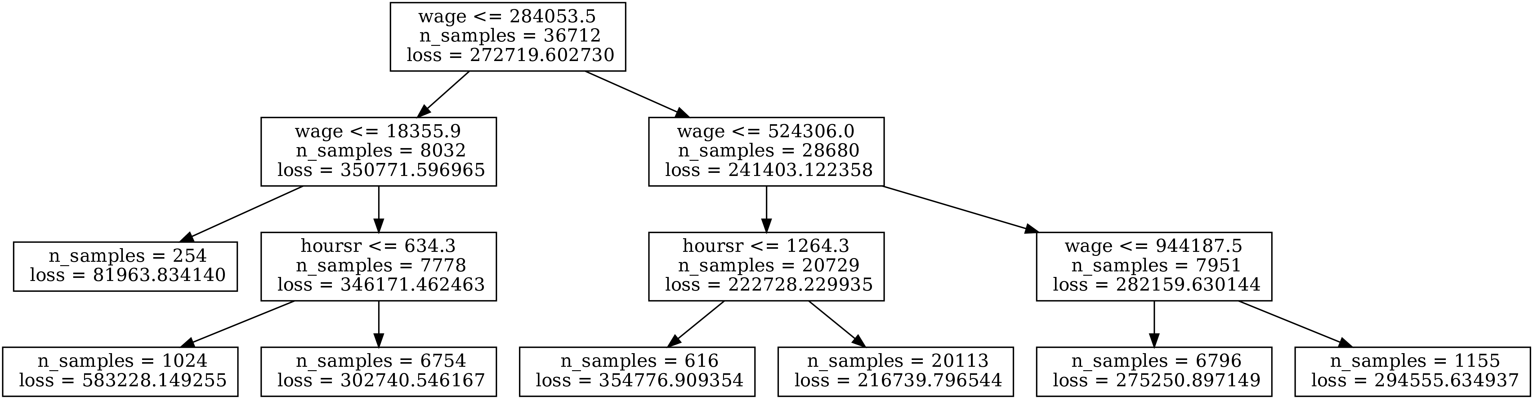
Figure: Figure A.1 – Regression Tree Structure for Men

7.4 Imputation Methodology

Because of the shortcomings of the contracted hours measure in the register data, we design an imputation approach that uses the Norwegian Labor Force Survey to obtain a better measure of hours worked. As we discuss in Sections 3.1 and A.3, this data set contains high quality survey data on actual hours worked but has a limited sample size. All individuals present in the Labor Force Survey are also present in the register data. We merge the two data sources using individual identification numbers and employ an imputation approach to infer actual hours worked for the entire population. In this section we explain our imputation approach in detail.

The Labor Force Survey records weekly hours worked. Each individual is surveyed up to eight consecutive quarters. We use only those who are present in all eight quarters and impute actual annual hours in year $t$ as: $h_{t}^{LFS}=13\cdot \sum _{q=1}^{4}h_{t,q}^{LFS}$, where $h_{t,d}^{LFS}$ is weekly hours in quarter $q$ of year $t$. We then employ a regression tree approach to estimate actual annual hours $h_{it}^{LFS}$ from the Labor Force Survey on information in the register data.

Classification and regression trees (CART) are widely used supervised machine-learning methods to develop prediction models because they are conceptually simple yet powerful. Tree-based methods recursively partition the training data space via feature threshold cuts into subsets with homogeneous values of the dependent variable, and then fit a simple prediction model within each partition. The classification tree algorithm is designed for fixed or categorical dependent variables, whereas regression trees are more suitable for predicting continuous dependent variables. CART algorithms are capable of handling a large number of features and observations and are easy to use.

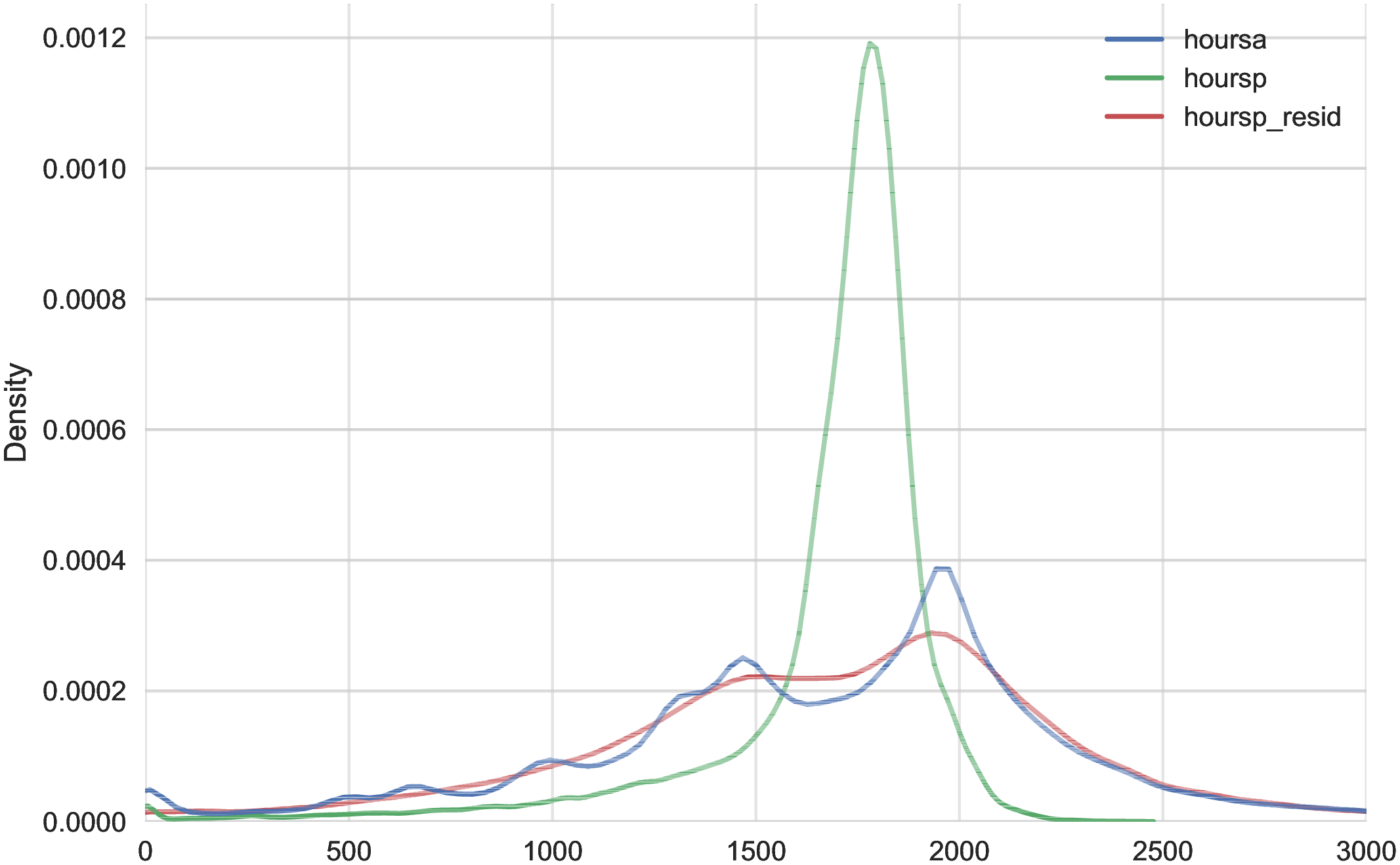
Figure A.2

–

Density of Imputed Hours versus Actual Hours

Note: The figure displays the kernel distribution of the actual annual hours in the Labor Force Survey and the kernel distribution of the imputed hours from the register data.

Figure: Figure A.2 – Density of Imputed Hours versus Actual Hours

The CART method employs a greedy search algorithm that starts with all the data. For each feature (i.e., predictor) it finds the split point that minimizes the weighted sum of squares of errors of the two models in two nodes. Then, the algorithm selects the best split point with the lowest loss value. Having found the best split, the algorithm then repeats the splitting process in each of the two partitions in the feature space. This process is then repeated recursively on all of the resulting regions until either a maximum level of depth or some minimum node size is reached. The schematic of this process looks like an inverted tree in which the root is on top while the leaves are at the bottom. After the tree is grown large, the algorithm then prunes some of the nodes to minimize the cross-validated sum of squares. For further details of the algorithm and its comparison with other tree-building procedures, see Hastie et al. (2009), Loh (2011), and Quinlan (1992).³⁷

Tree size is a tuning parameter governing the model’s complexity. Clearly a too large tree might overfit the data (i.e. poor out of sample prediction), while a small tree might not capture the important structure. Thus, we choose this tuning parameter to minimize the sum of squared errors for the test sample.

When branching the data to grow a complete tree, we develop a regression model at each node for prediction:³⁸

\[ h_{it}^{LFS}=\beta X_{it}+\epsilon _{it}. \] We use a a rich set of regressors, $X_{it}$, from the register data (the Labor and Welfare Administration Register and the Administrative Tax and Income Records). In particular, we include contractual hours, sickness days, parental leave days, and unemployment days reported in the Employment Register as well as their change from last year as these are informative about total hours worked in the current year. We also include earnings from the tax and income records as a an explanatory variable. Earnings contain valuable information which our other variables do not capture. It does for example covary with overtime.³⁹ To capture the impact of job characteristics on hours worked, we include indicator variables for part-time versus full-time and public versus private sector employment as well as their change from the last year. The change variables can take three possible values: $-1$, $0$, and $1$. Job change is an important predictor for labor supply (see Guvenen et al. (2019)), thus we include indicator variables for job stayers in the current year and the last year. Life-cycle variation and educational differences in labor supply are well known (see e.g. Chakraborty et al. (2015), Bick et al. (2022)), therefore, these variables are covered in our set of regressors. In particular, we use three age groups and three education groups in our model. We further include marital status and its change since last year as independent variables (see e.g. Chakraborty et al. (2015) for variation in labor supply by marital status). Finally, we include average past earnings, current annual earnings and arc percent change in annual earnings as additional regressors.⁴⁰

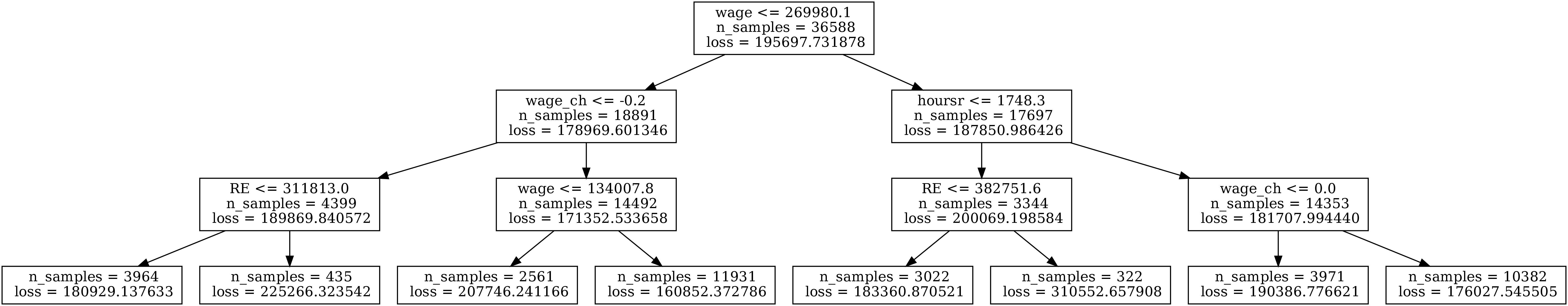
Figure: Figure A.3 – Regression Tree Structure for Women

				Node
Regressor	1	2	3	4	5	6	7
Constant	891.92	-1475.56	-971.71	-1537.20	-1426.08	-222.24	-6623.32
Earnings/1000	8.89	2.88	1.97	0.40	0.74	0.43	0.03
Earnings Change	49.92	-98.29	94.29	150.35	175.56	14.41	34.30
Register hours	0.04	0.07	0.18	-0.10	0.28	0.18	0.15
Register hours change	-87.41	36.66	-18.02	43.21	-58.57	27.88	-27.12
Married	17.85	176.62	8.86	-51.55	-21.76	-64.85	81.88
Public employee	-7.10	43.10	-120.94	74.07	-83.10	45.38	164.95
Frac. Non-parent days	-627.33	154.12	263.36	-215.09	675.38	566.51	-333.63
Frac. Non-sick days	-144.05	1034.69	900.25	2245.30	1066.29	250.25	5152.95
Frac. Empl. days	-96.57	189.38	139.83	337.02	385.41	-106.86	-660.08
Frac. Tot. Emp. days.	130.25	857.06	648.41	1352.76	402.36	1055.66	4159.24
Part-time job	-118.90	-64.29	-29.01	27.78	-8.06	-30.01	-59.12
Change in marriage	271.90	-118.01	-75.19	138.78	0.77	124.91	120.18
Change in public emp.	-121.36	-33.05	15.95	-175.00	40.67	-9.78	118.59
Change in part-time job	27.45	47.62	-0.54	-80.55	-17.07	-29.21	13.08
Ch. Frac. Non-parent days	178.30	1012.53	-119.26	-220.72	-101.81	128.01	617.59
Ch. Frac. Non-sick days	-71.25	-412.61	-446.23	-913.63	-102.44	750.61	-2875.70
Ch. Frac. Emp. days	60.56	481.39	4.40	6.28	234.72	610.17	675.30
Ch. Frac. Tot. Emp. days.	-10.75	-523.44	-28.15	-107.11	-159.56	-648.60	-1582.80
Recent earnings/1000	0.08	-0.18	-0.30	-0.19	-0.27	-0.25	-0.02
Job stayer	-109.93	103.20	-21.35	-123.22	-22.65	18.50	-84.38
Job stayer last year	-5.26	-27.50	-41.99	6.53	-25.77	-34.37	-57.56
Primary Educ (reference)	0.00	0.00	0.00	0.00	0.00	0.00	0.00
Upper secondary	73.08	102.51	9.61	-155.20	7.31	-90.73	120.53
College/university	-4.67	89.03	-57.52	-368.94	-38.31	-99.27	62.01
Agebin	-7.33	-17.40	-3.85	-46.23	-0.87	-12.81	-11.36
R - squared	0.15	0.22	0.27	0.27	0.05	0.03	0.05
No. of observations	254	1024	6754	616	20113	6795	1156
			p < 0.05,	** p < 0.01

Table A.3 – Regression Tree Results (Men)

Note:

The table displays the coefficients from the regression of male hours from the Norwegian Labor Force Survey on observables

in the register data at each of the terminal nodes in the regression tree in Figure A.1.

Since we also include the change for some of our variables (between $t$ and $t+1$) we drop observations before 2004. We require each individual to have at least three years of non-missing earnings observations between $t-1$ and $t-5$ to construct average recent earnings. For the small number of workers who have self employment income above the minimum income threshold $Y_{\text{min},t}$ and labor earnings less than $Y_{\text{min},t}$, we set actual hours to zero because in our empirical analysis we only include wage and salary workers. Again, for the small number of workers who have labor earnings less than half of $Y_{\text{min},t}$ and $Y_{\text{min},t}$, we winsorize their actual hours at 130 and 260, respectively. We divide the sickness days, parental leave days, and unemployment days reported in the Employment Register by 365 to normalize their values.

To select the optimal regression tree structure we experiment with various depths of the tree (up to five layers) and evaluate the goodness of fit in the training sample as well as an out-of-sample test sample. To do so, as is standard in the machine learning literature, we use 80% of our sample to fit the model and the rest to evaluate the performance out of sample. In general, choosing a deeper tree with finer categories will increase the in-sample fit but may come at the cost of overfitting, which will decrease the accuracy of out-of-sample predictions.

We estimate the model separately for men and women. Table I summarizes the $R^{2}$ in the training sample and test sample for different depths of the tree. Figures A.1 and A.3 show these tree structures and the coefficients of linear regression models are reported in Tables A.3 and A.4.⁴¹ We use these estimated models to impute actual work hours for the individuals that are not present in the Labor Force Survey.

We have experimented with alternative methodologies and models, such as neural networks, LASSO, quantile regression, regression in growth instead of levels, allowing for more interaction between the explanatory variables, and other forms of more flexible parameterization. In the end, none of these alternatives outperformed the regression tree model in terms of explanatory power and out-of-sample prediction.

				Node
Regressor	1	2	3	4	5	6	7
Constant	-160.62	-1148.43	-775.60	-1028.75	-1343.24	-1479.40	2411.08
Earnings/1000	3.09	1.10	5.38	3.25	0.75	0.88	0.37
Earnings Change	156.84	242.02	32.73	40.36	64.53	264.69	661.42
Register hours	0.07	-0.03	0.12	0.24	0.03	-0.03	0.20
Register hours change	-2.64	122.93	-15.93	-12.55	-47.44	-12.90	28.41
Married	-79.21	-193.25	-26.43	-19.11	-70.98	-33.97	-60.71
Public employee	4.72	41.95	-8.95	-55.03	-56.70	182.51	-65.86
Frac. Non-parent days	419.66	874.38	382.86	653.44	1048.50	818.15	-154.53
Frac. Non-sick days	59.59	937.28	423.74	432.80	1077.12	769.61	-1473.04
Frac. Empl. days	5.27	855.06	48.79	72.30	517.19	41.24	-2336.01
Frac. Tot. Emp. days.	200.28	-497.01	209.24	313.53	151.27	1479.60	2876.41
Part-time job	52.42	343.50	-30.81	42.04	67.57	50.43	100.60
Change in marriage	-22.92	436.91	-120.52	9.48	120.78	-3.36	-16.83
Change in public emp.	-21.92	-159.50	3.49	5.18	24.14	-220.14	-13.42
Change in part-time job	-65.99	-54.93	25.32	-42.67	-51.94	-82.65	-90.41
Ch. Frac. Non-parent days	-277.59	-498.36	-38.93	-73.32	-16.84	-617.07	-998.92
Ch. Frac. Non-sick days	-63.09	-1005.95	-110.66	-221.51	-203.85	-466.76	-488.23
Ch. Frac. Emp. days	122.01	-449.30	148.05	183.21	184.64	543.84	501.46
Ch. Frac. Tot. Emp. days.	-73.07	620.70	-151.14	-90.42	-126.90	-689.40	-137.82
Recent earnings/1000	0.01	0.30	-0.52	-0.11	-0.21	-0.82	0.10
Job stayer	-72.36	14.70	-21.92	-20.69	-49.93	-163.34	-30.55
Job stayer last year	-4.49	12.09	-2.79	-29.26	-25.76	-49.65	-34.27
Primary Educ (reference)	0.00	0.00	0.00	0.00	0.00	0.00	0.00
Upper secondary	11.65	-265.72	6.04	-22.18	-0.30	-45.07	-25.01
College/university	-38.52	-312.95	34.36	-136.80	-93.23	-127.70	-69.44
Agebin	5.98	45.07	-7.34	-18.29	-18.27	73.68	-17.50
R - squared	0.38	0.28	0.19	0.269	0.06	0.28	0.12
No. of observations	3932	434	2569	11955	3022	322	3392
			p < 0.05,	** p < 0.01

Table A.4 – Regression Tree Results (Women)

Note:

The table displays the coefficients from the regression of female hours from the Norwegian Labor Force Survey on

observables in the register data at each of the terminal nodes in the regression tree in Figure A.4.

8 Additional Figures and Tables

8.1 Moments of Earnings Growth: Norway vs. the U.S.

(a) Variance

(b) Skewness

Figure B.1 – Cross-Sectional Moments of One-Year Log Earnings Growth in the U.S.

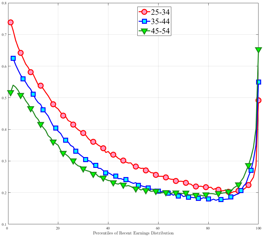
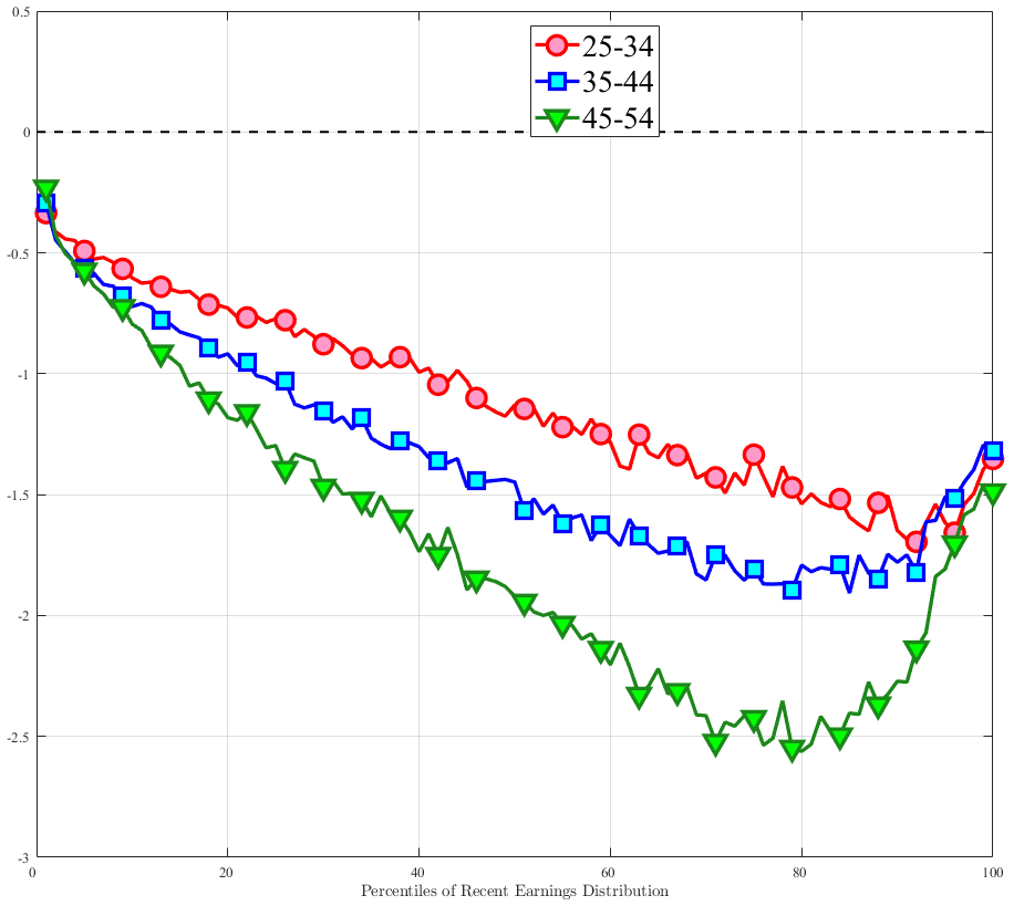
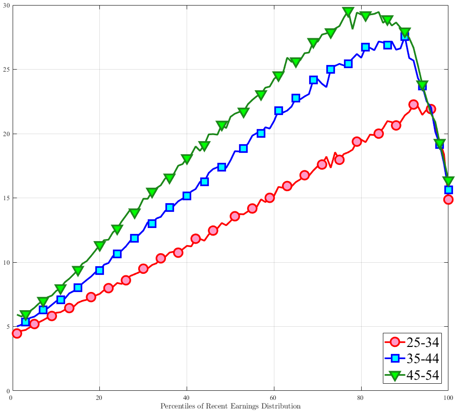
Note: The figure displays the higher-order moments of one-year earnings growth ($y_{t+1}-y_{t}$) for three age groups in the U.S. Source: Guvenen et al. (2019). Each point on these figures represents one percentile of RE.

(a) Standard Deviation

(b) Skewness

Figure B.2 – Cross-Sectional Moments of Five-Year Log Earnings Growth in the U.S.

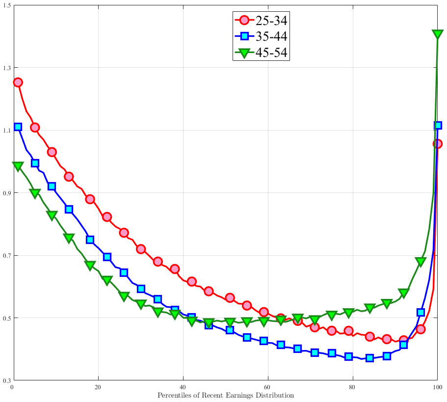
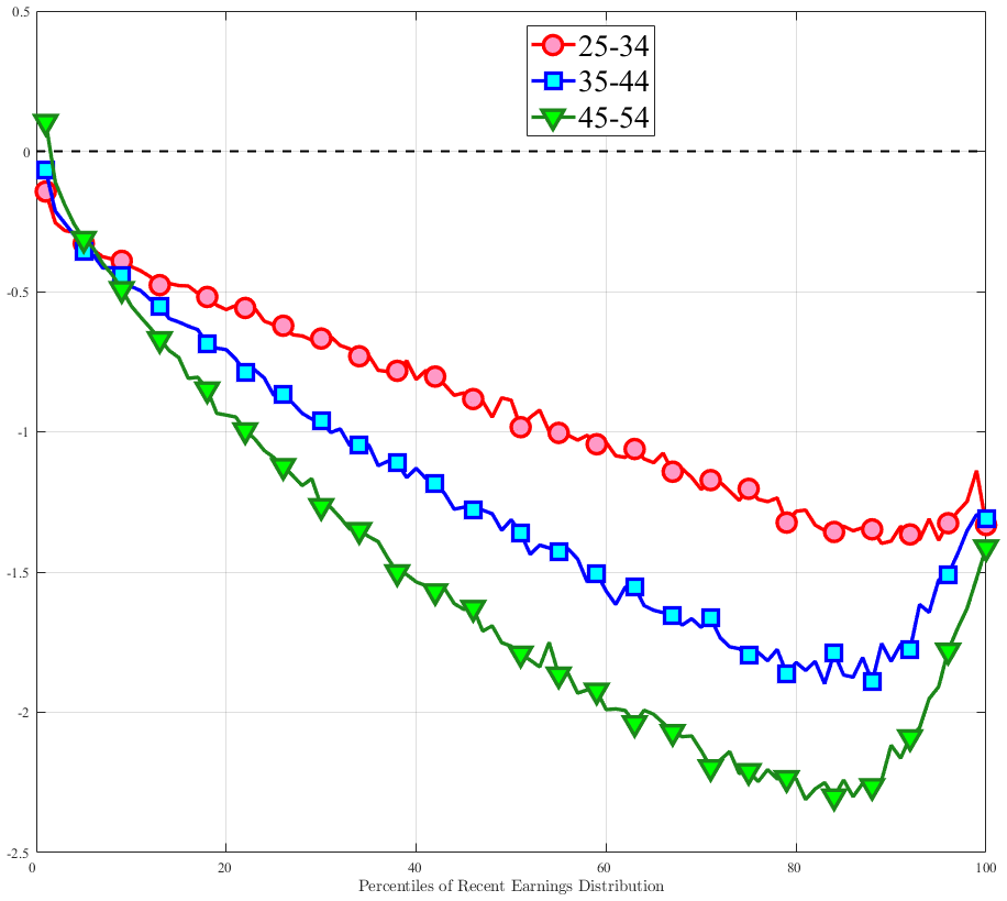
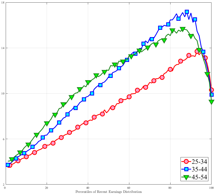
Note: The figure displays the higher-order moments of five-year earnings growth ($y_{t+5}-y_{t}$) for three age groups in the U.S. Source: Guvenen et al. (2019). Each point on these figures represents one percentile.

(a) Variance

(b) Skewness

Figure B.3 – Cross-Sectional Moments of One-Year Log Earnings Growth in Norway

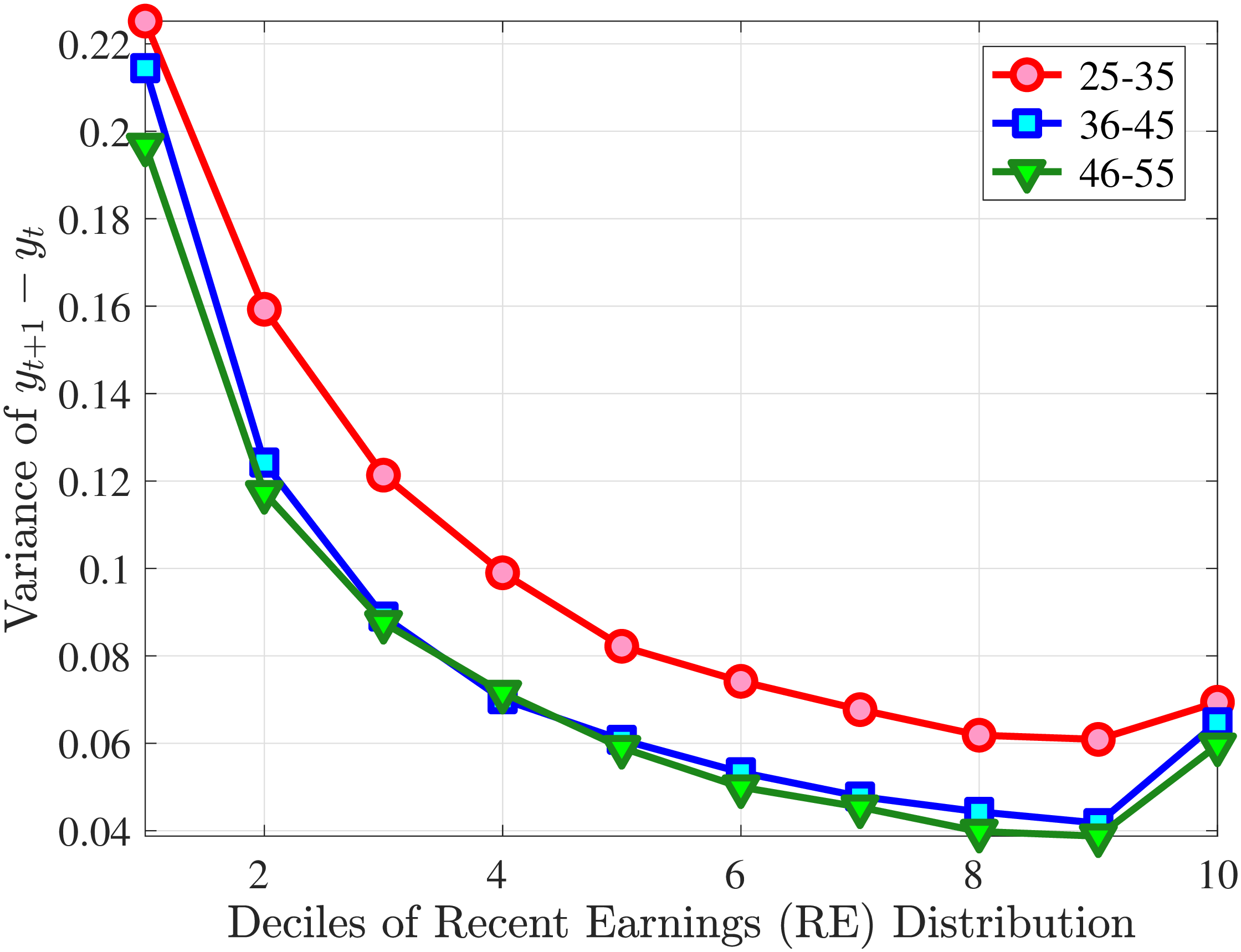
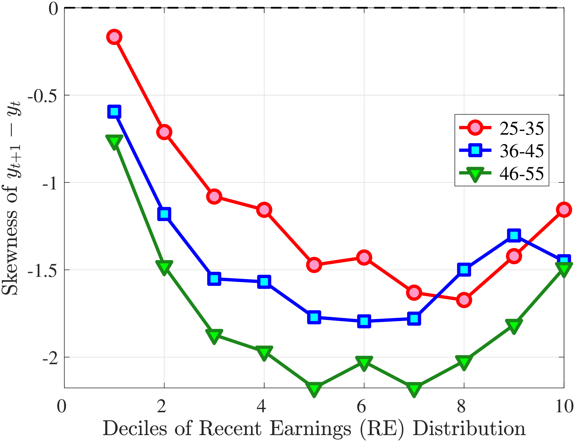
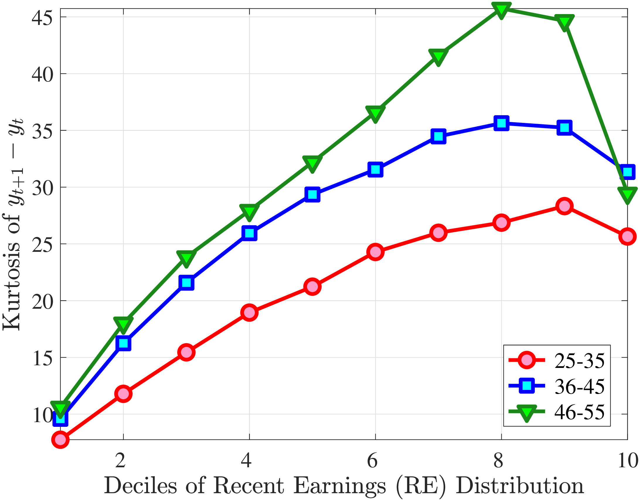
Note: The figure displays higher-order moments of one-year earnings growth ($y_{t+1}-y_{t}$) for three age groups in Norway.

(a) Variance

(b) Skewness

Figure B.4 – Cross-Sectional Moments of Five-Year Log Earnings Growth in Norway

Note: The figure displays higher-order moments of five-year earnings growth ($y_{t+5}-y_{t}$) for three age groups in Norway.

Figure B.5 – Kelly Skewness of Earnings Growth for Males

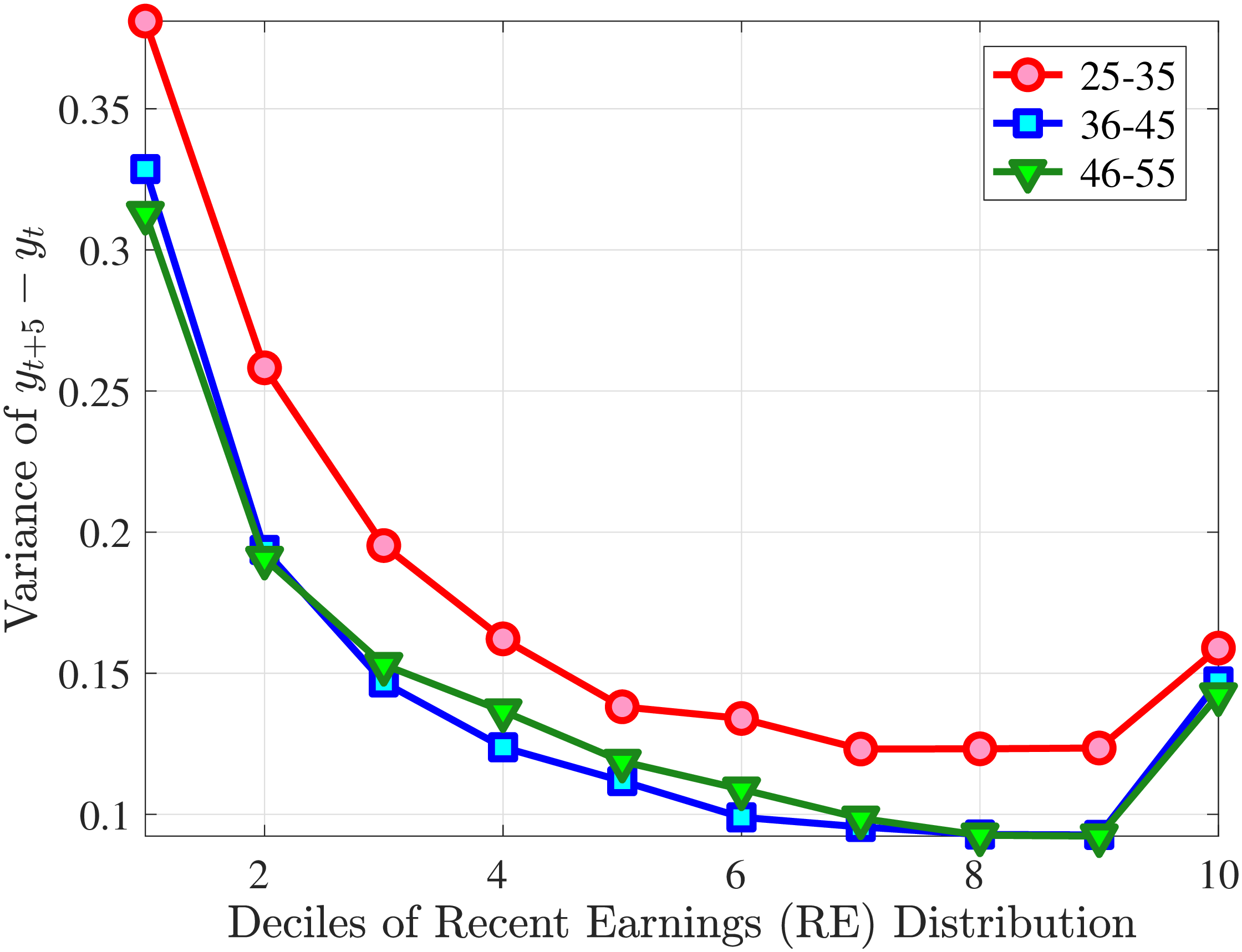
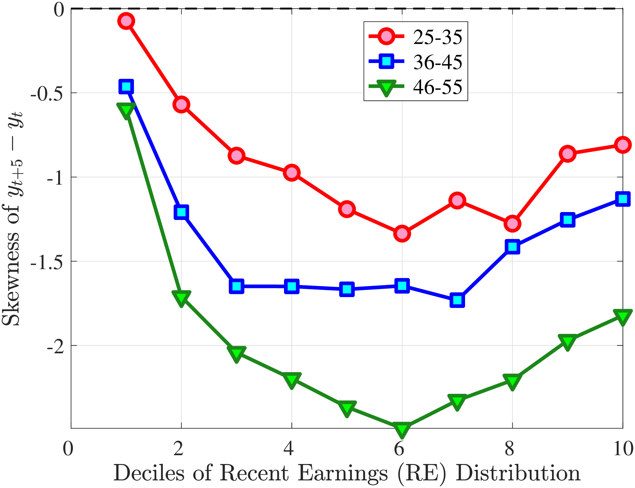
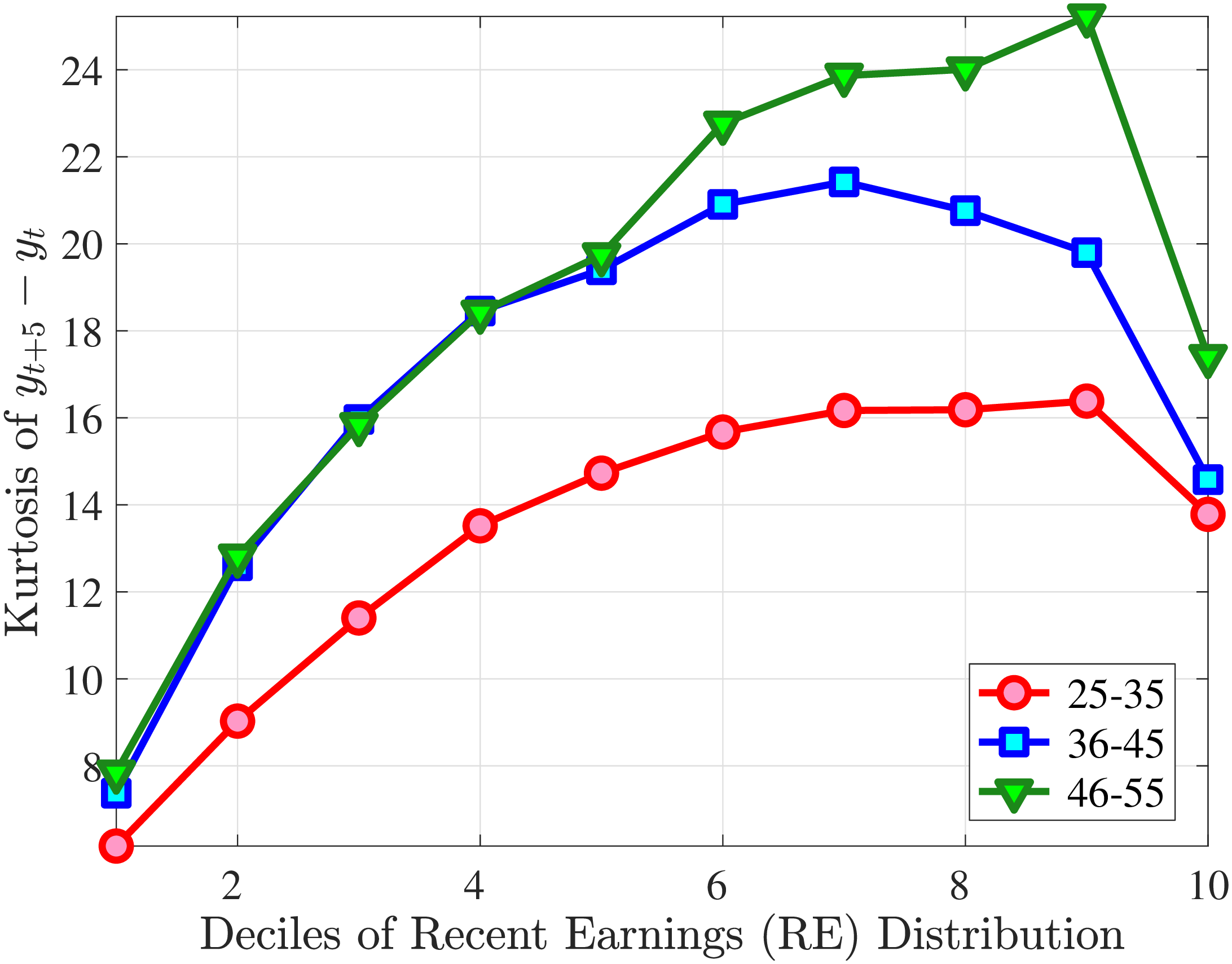
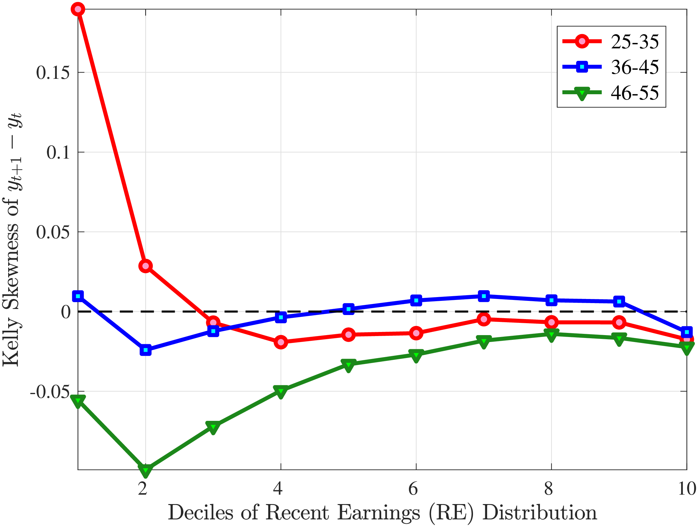
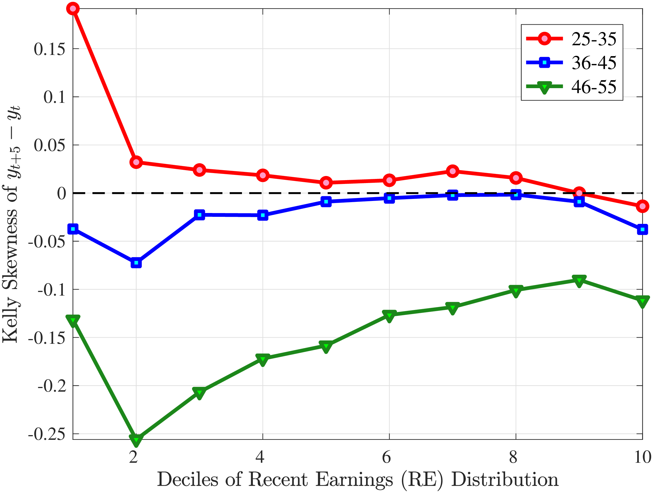
Note: The figure displays Kelly skewness for five-year earnings growth (left panel) and five-year earnings growth (right panel) for three age groups in Norway.

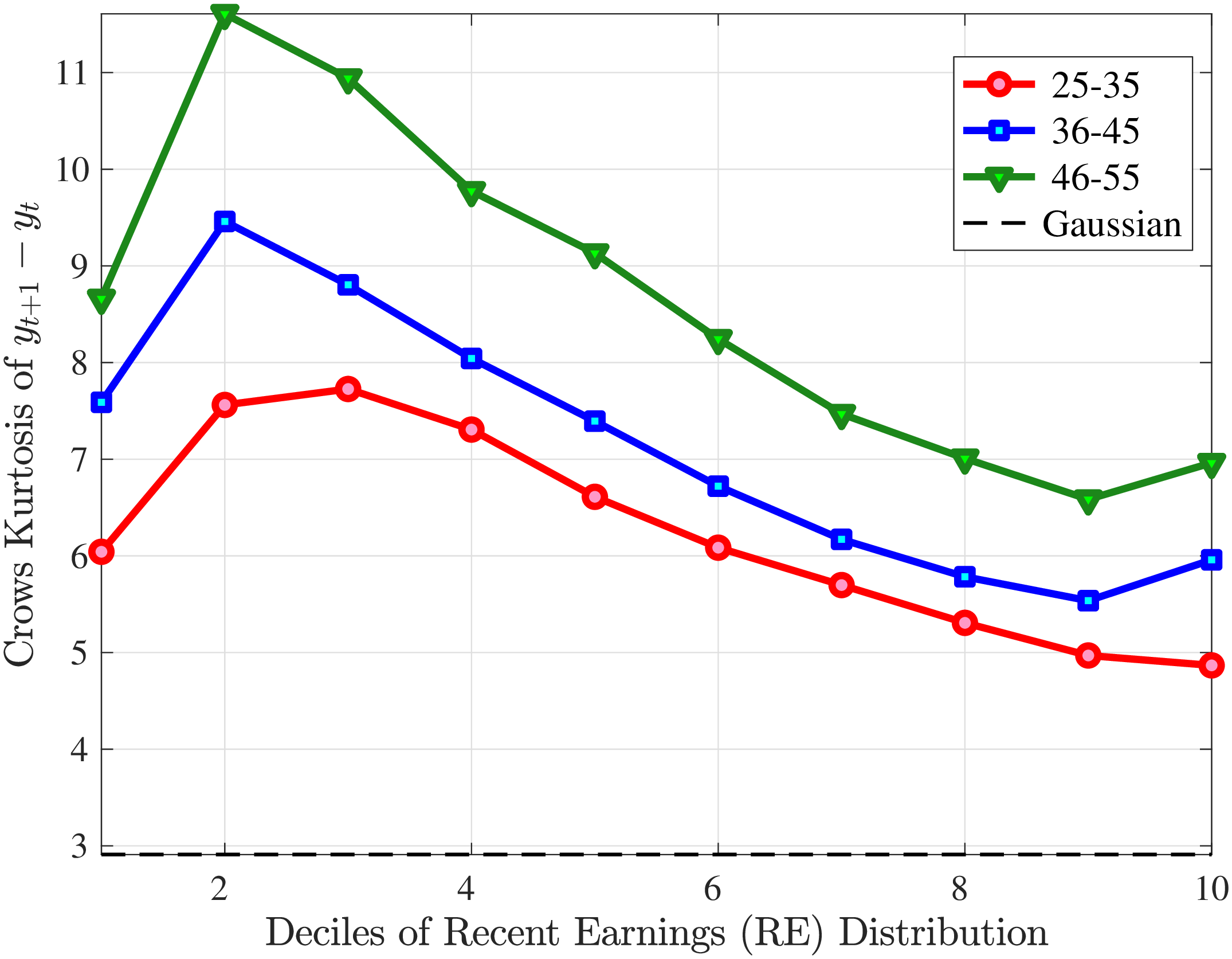
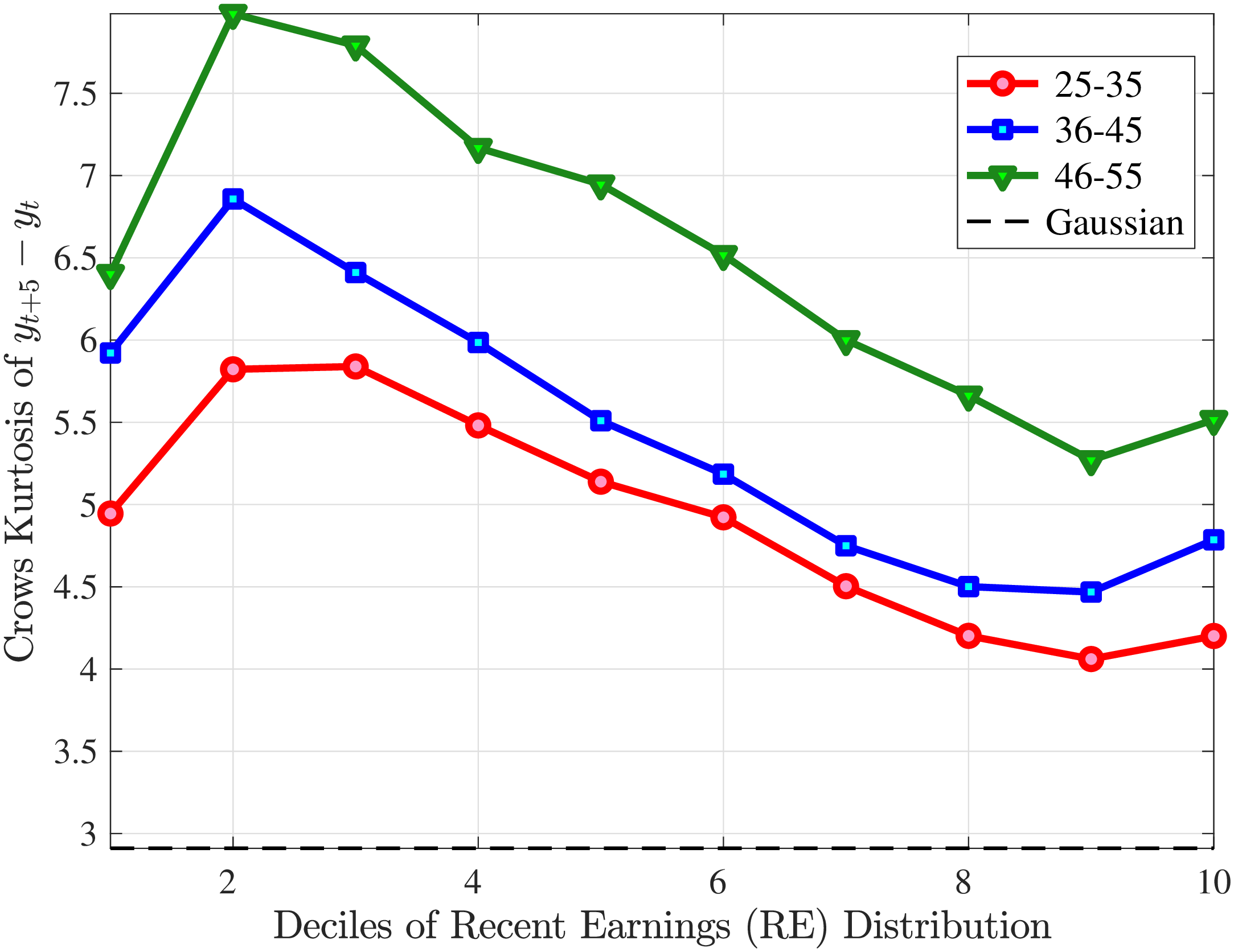
Figure B.6 – Crow-Siddiqui Kurtosis of Earnings Growth for Males

Note: The figure displays Crow-Siddiqui kurtosis for one-year earnings growth (left panel) and five-year earnings growth (right panel) for three age groups in Norway.

8.2 Decomposing Earnings Growth into Hours and Wages

2nd RE Decile

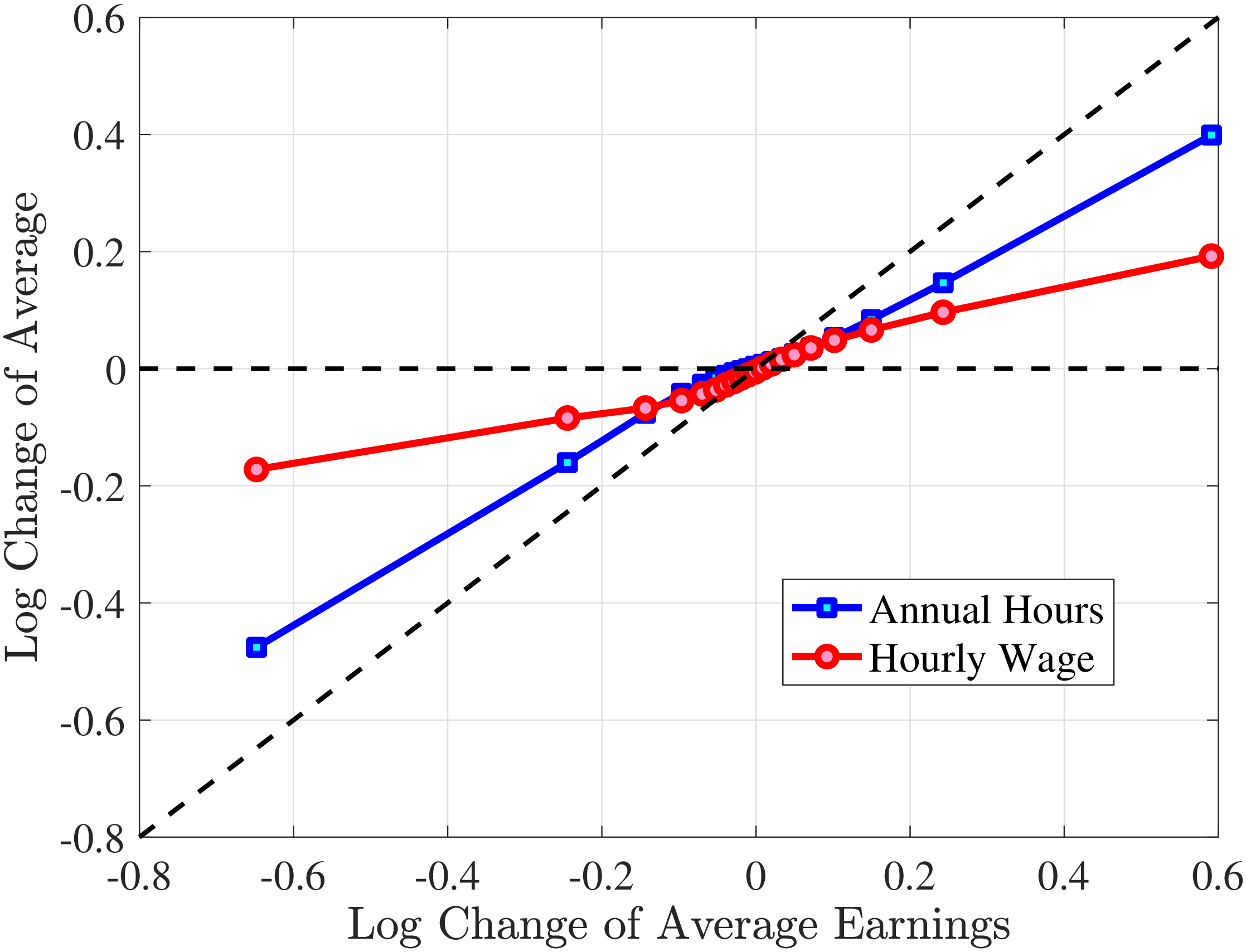
3rd RE Decile

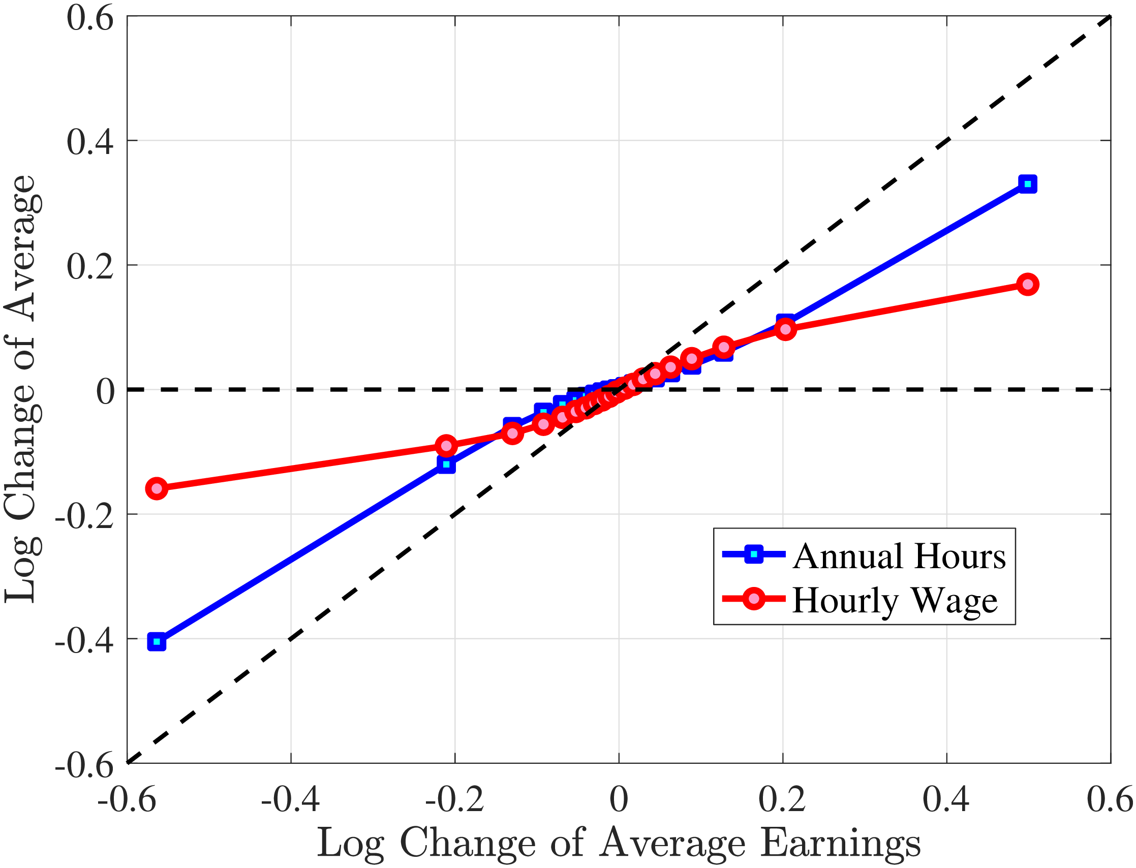
Figure B.7

–

Contributions of Hours and Wage Rates to Earnings Shocks

Note: The figure displays the one-year Representative-Agent changes (log change of averages) for imputed hours and imputed wage rates for 20 different groups of prime-age males (ages 36 to 55) in the 2nd RE decile (left panel) and 3rd RE decile (right panel), plotted against their contemporaneous one-year log change in average annual earnings.

Figure: Figure B.7 – Contributions of Hours and Wage Rates to Earnings Shocks

8th RE Decile

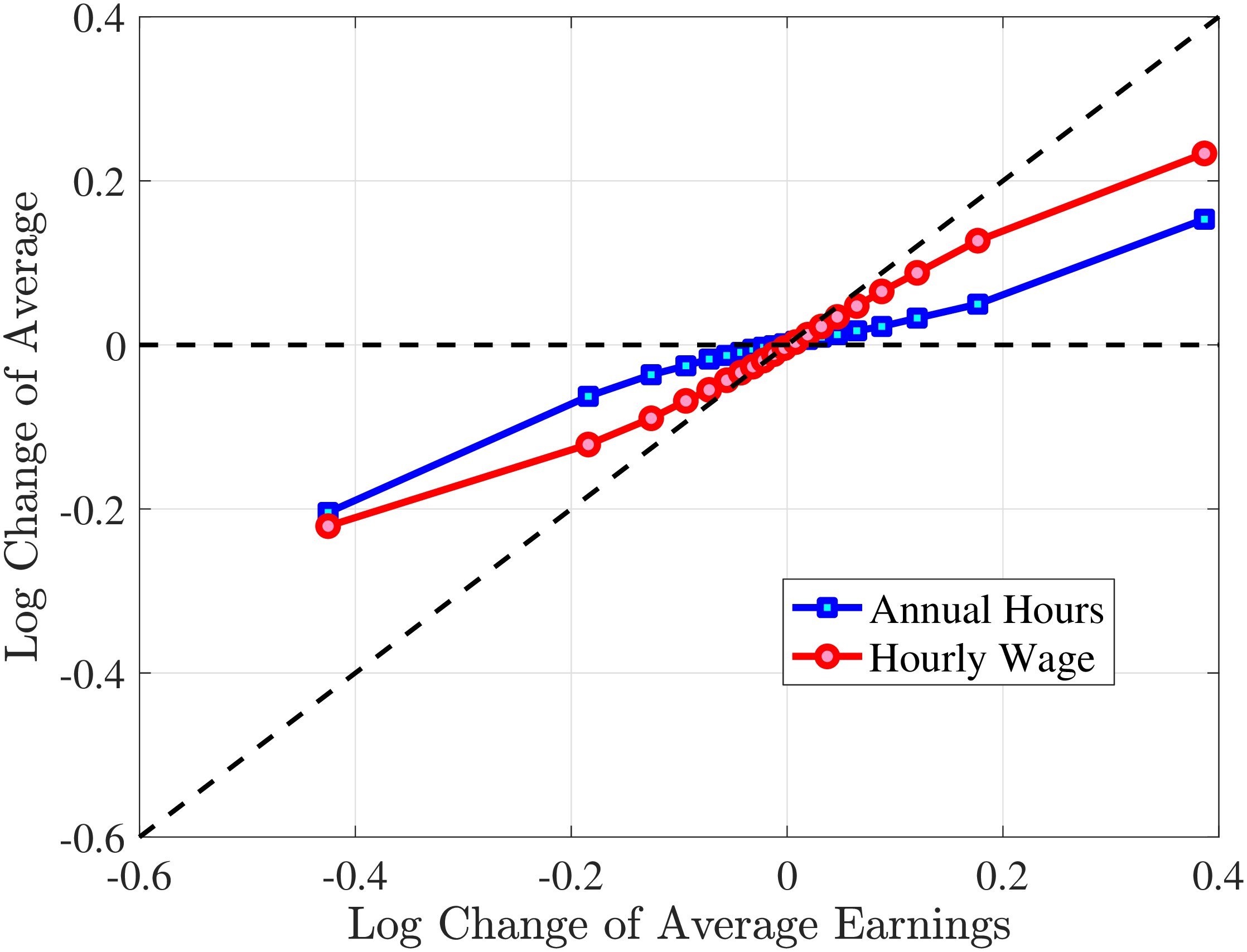
9th RE Decile

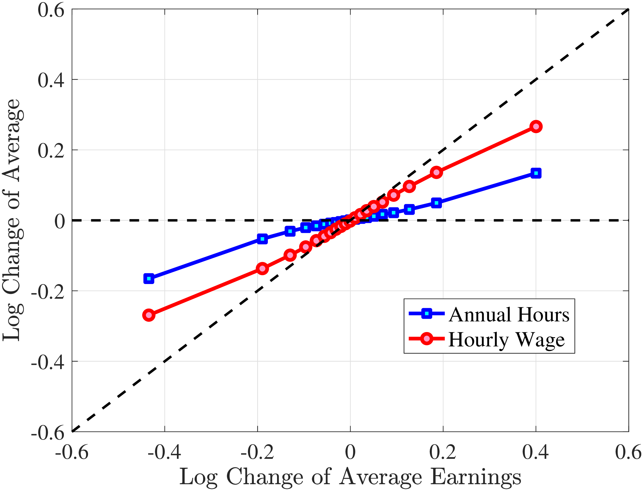
Figure B.8

–

Contributions of Hours and Wage Rates to Earnings Shocks

Note: The figure displays the one-year Representative-Agent changes (log change of averages) for imputed hours and imputed wage rates for 20 different groups of prime-age males (ages 36 to 55) in the 8th RE decile (left panel) and 9th RE decile (right panel), plotted against their contemporaneous one-year log change in average annual earnings.

Figure: Figure B.8 – Contributions of Hours and Wage Rates to Earnings Shocks

8.3 Additional Moments of Male Hours and Wage Growth

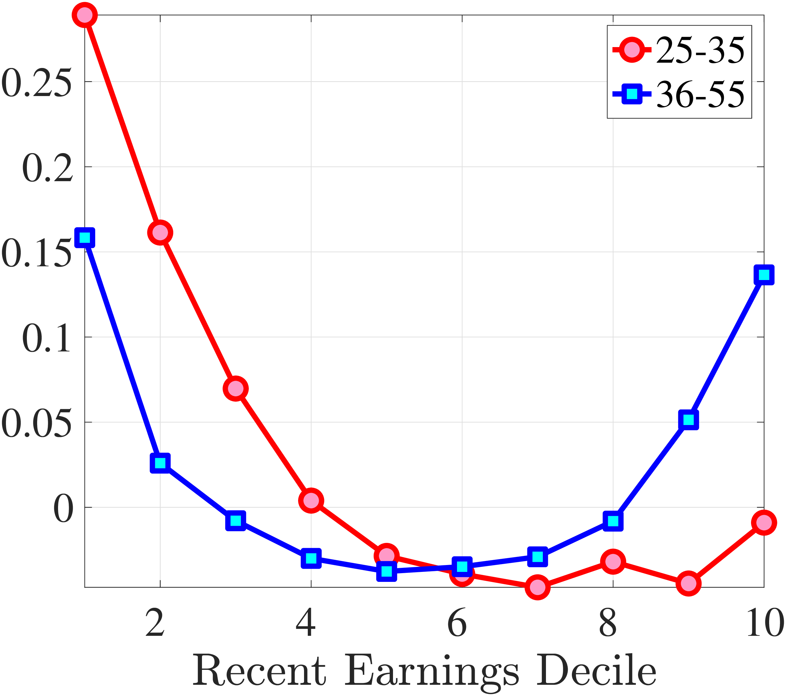(a) One-Year Hours Growth 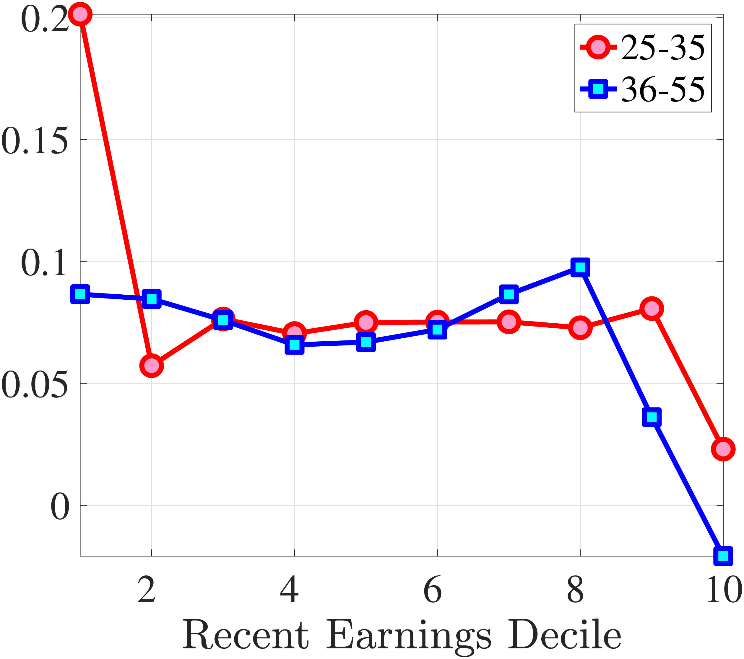(b) One-Year Hourly Wage Rate Growth

Figure B.9

–

Kelly Skewness of One-Year Male Hours and Hourly Wage Growth

Note: The figure displays Kelly skewness for one-year hours growth (left panel) and one-year hourly wage rate growth (right panel) for two age groups in Norway.

Figure: Figure B.9 – Kelly Skewness of One-Year Male Hours and Hourly Wage Growth

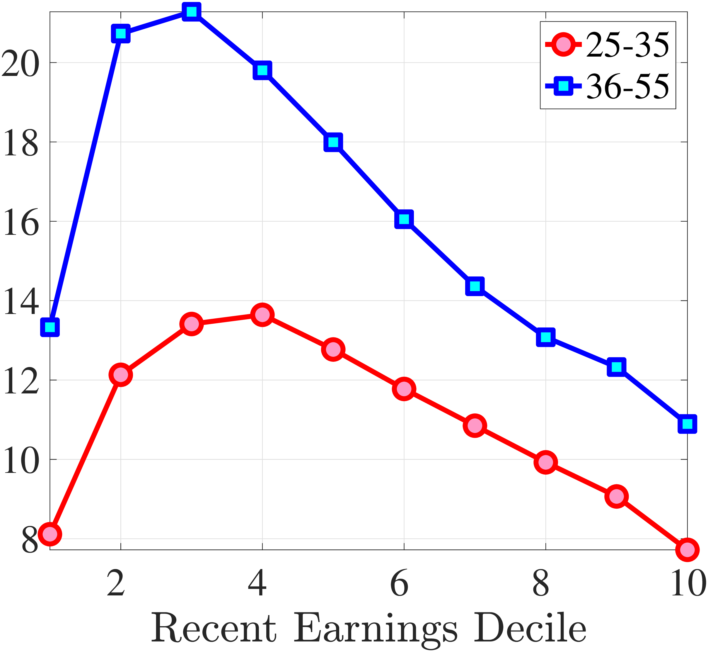(a) One-Year Hours Growth 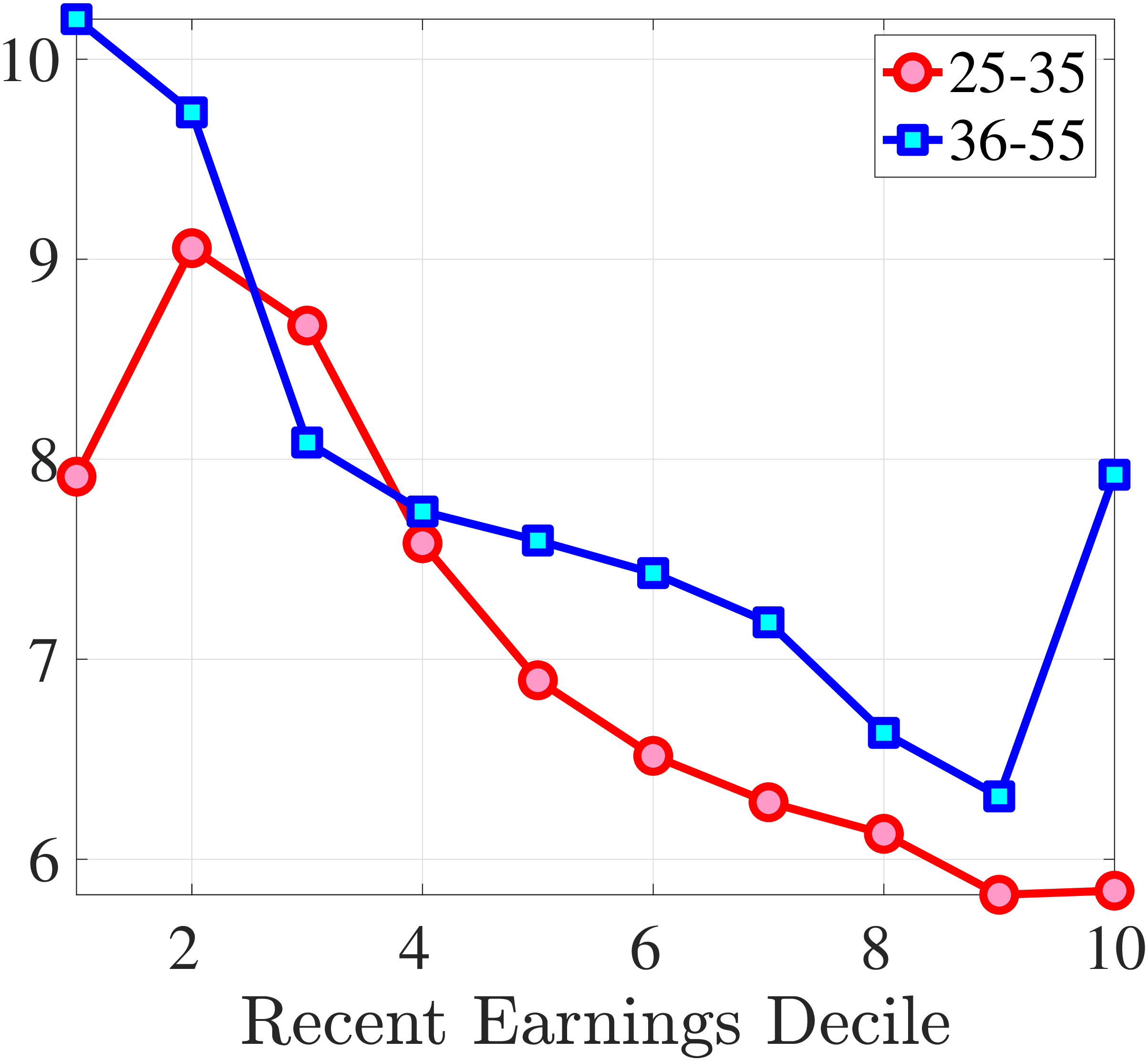(b) One-Year Hourly Wage Rate Growth

Figure B.10

–

Crow-Siddiqui Kurtosis of One-Year Male Hours and Hourly Wage Growth

Note: The figure displays Crow-Siddiqui kurtosis for one-year hours growth (left panel) and one-year hourly wage rate growth (right panel) for two age groups in Norway.

Figure: Figure B.10 – Crow-Siddiqui Kurtosis of One-Year Male Hours and Hourly Wage Growth

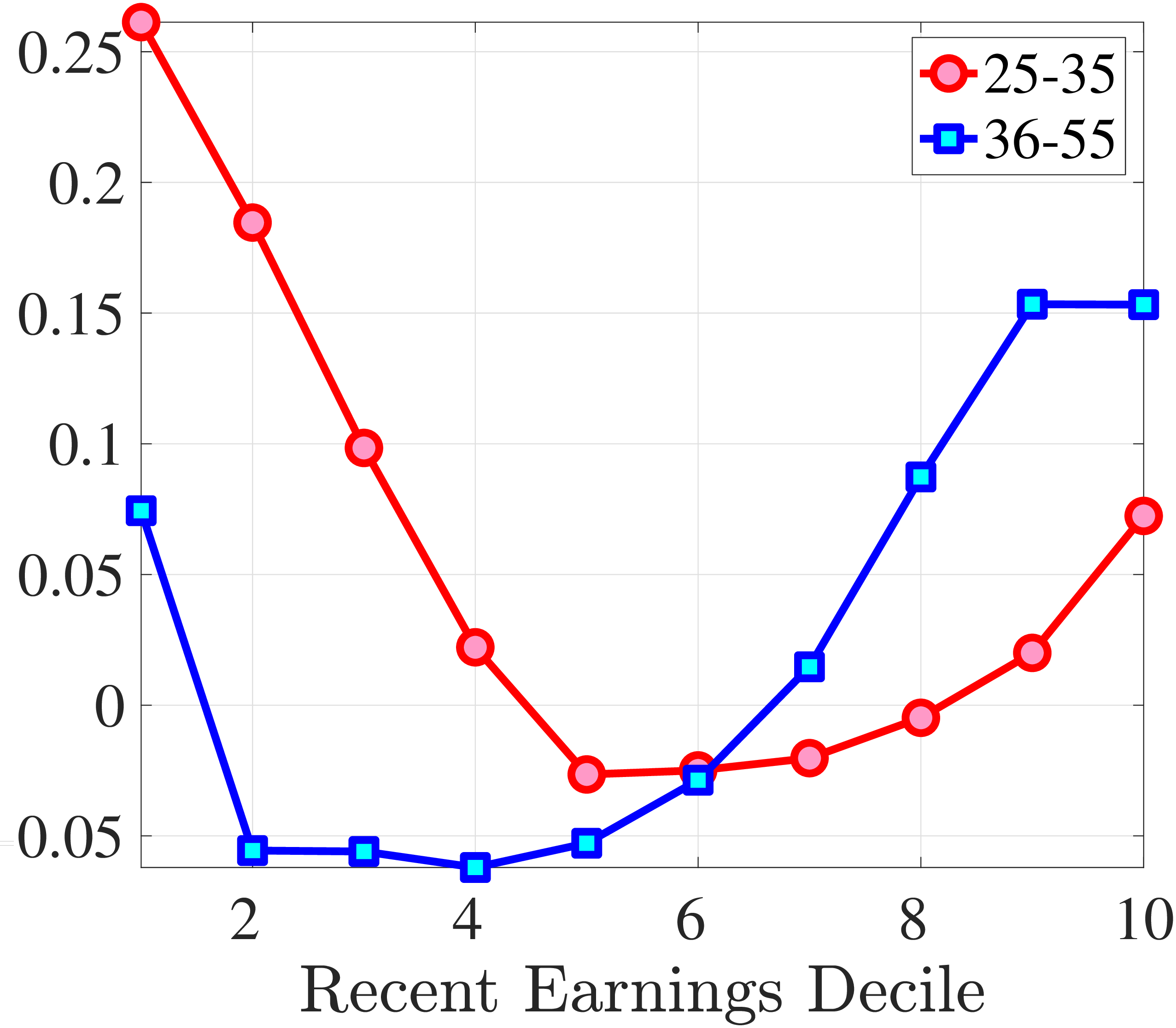(a) Five-Year Hours Growth 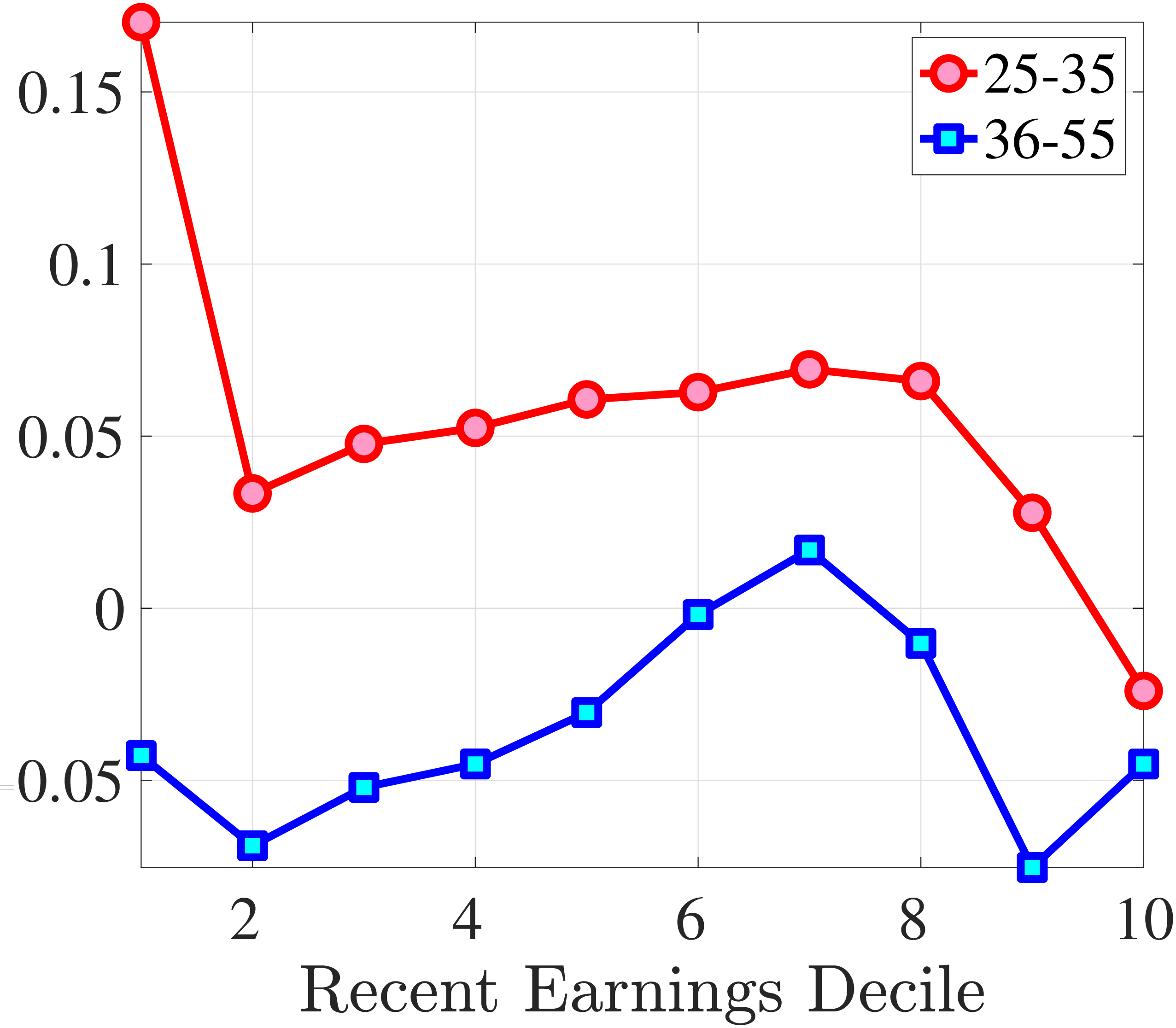(b) Five-Year Hourly Wage Rate Growth

Figure B.11

–

Kelly Skewness of Five-Year Male Hours and Hourly Wage Growth

Note: The figure displays Kelly skewness for five-year hours growth (left panel) and one-year hourly wage rate growth (right panel) for two age groups in Norway.

Figure: Figure B.11 – Kelly Skewness of Five-Year Male Hours and Hourly Wage Growth

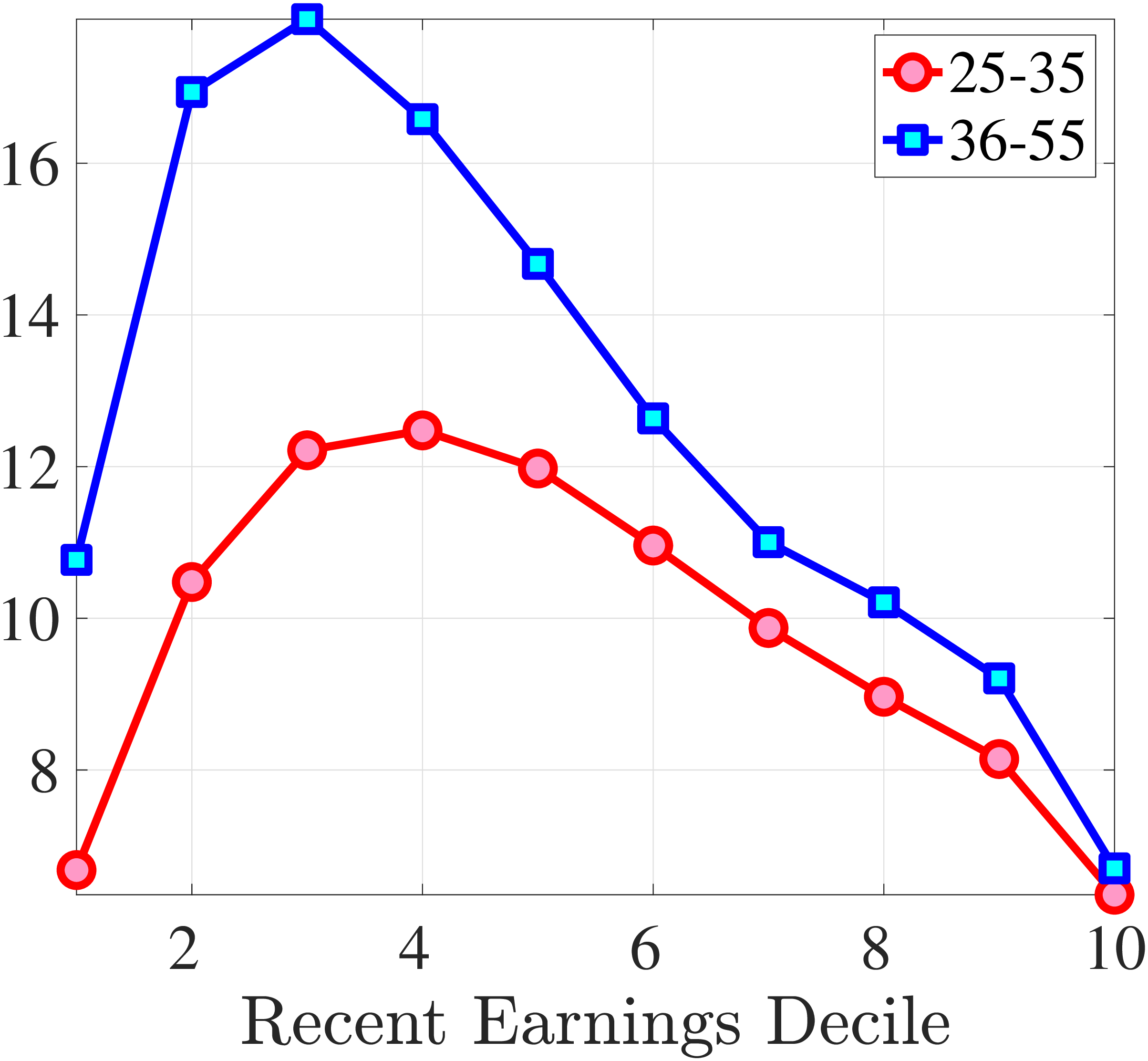(a) Five-Year Hours Growth 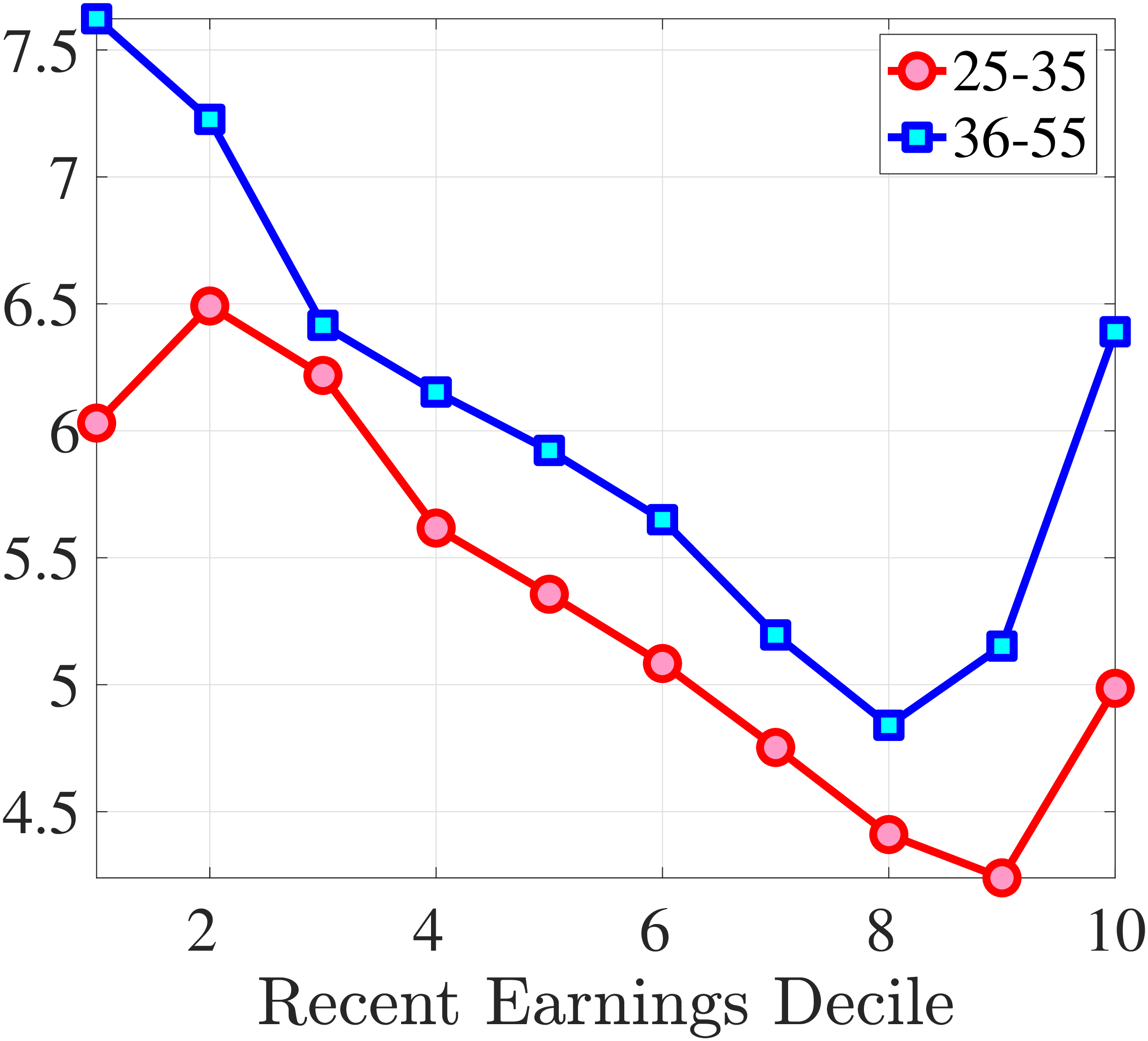(b) Five-Year Hourly Wage Growth

Figure B.12

–

Crow-Siddiqui Kurtosis of Five -Year Male Hours and Hourly Wage Growth

Note: The figure displays Crow-Siddiqui kurtosis for five-year hours growth (left panel) and one-year hourly wage rate growth (right panel) for two age groups in Norway.

Figure: Figure B.12 – Crow-Siddiqui Kurtosis of Five -Year Male Hours and Hourly Wage Growth

8.4 Additional Figures for Decomposition of Moments

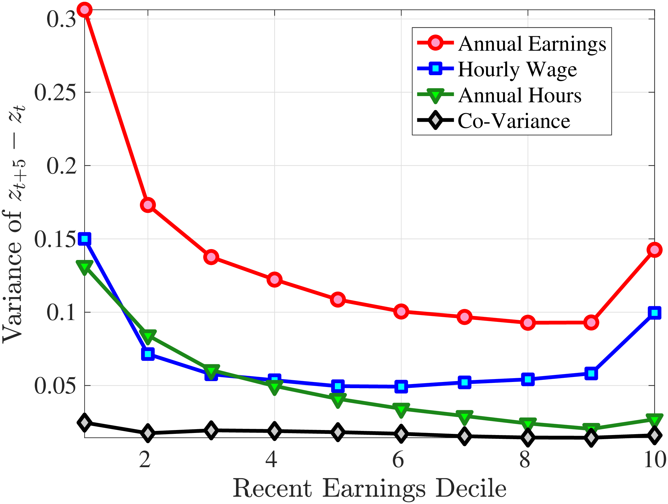(a) Prime-Age Workers: 36–55 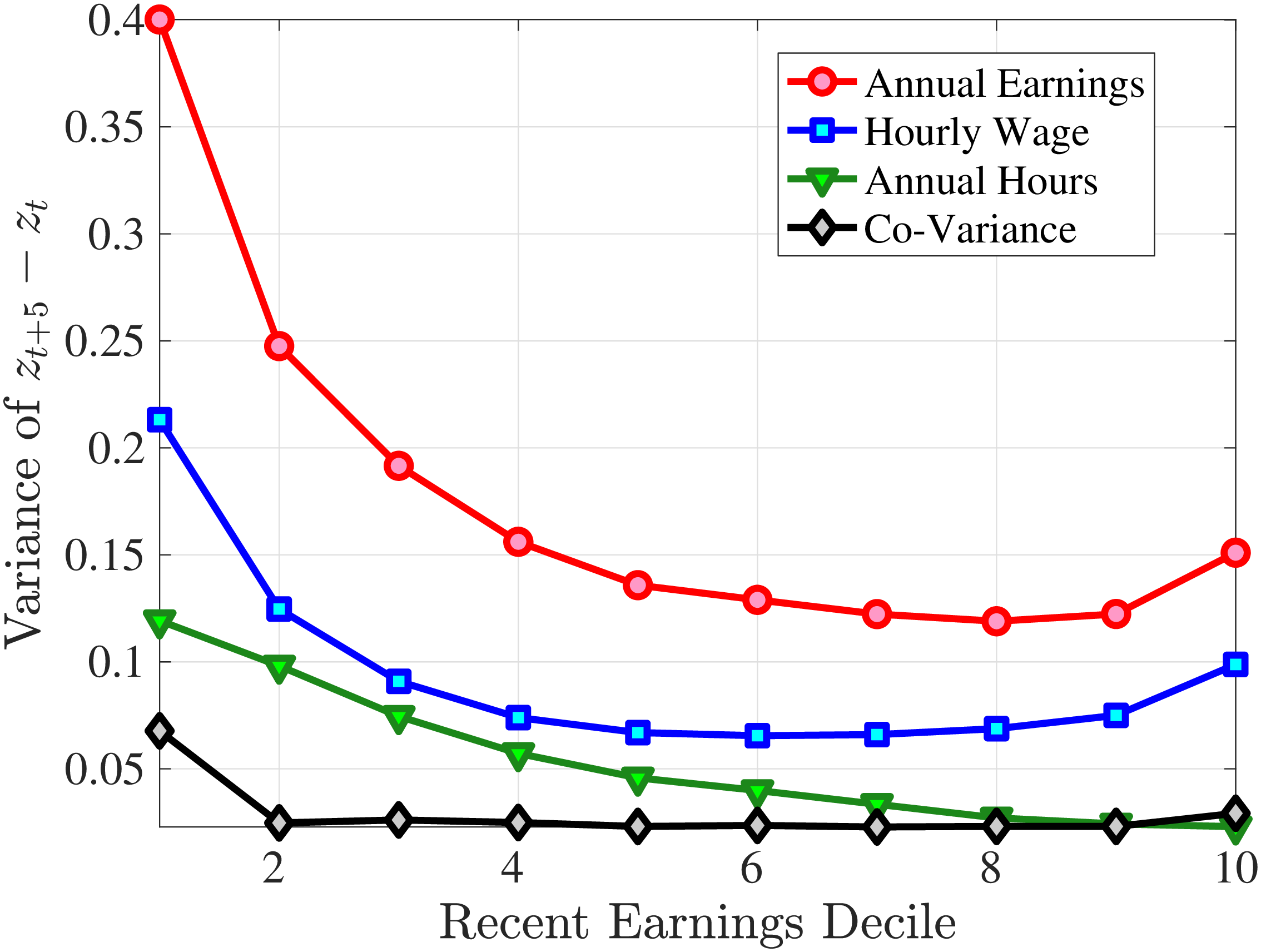(b) Young Workers: 25–35

Figure B.13

–

Decomposition of Variance of Five-Year Growth

Note: The figure decomposes the variance of five-year log earnings changes (red line) into the variance of log wage changes (blue line), the variance of log hours changes (green line), and the co-variance between log wage and log hours changes (black line). Each dot represents a decile of RE.

Figure: Figure B.13 – Decomposition of Variance of Five-Year Growth

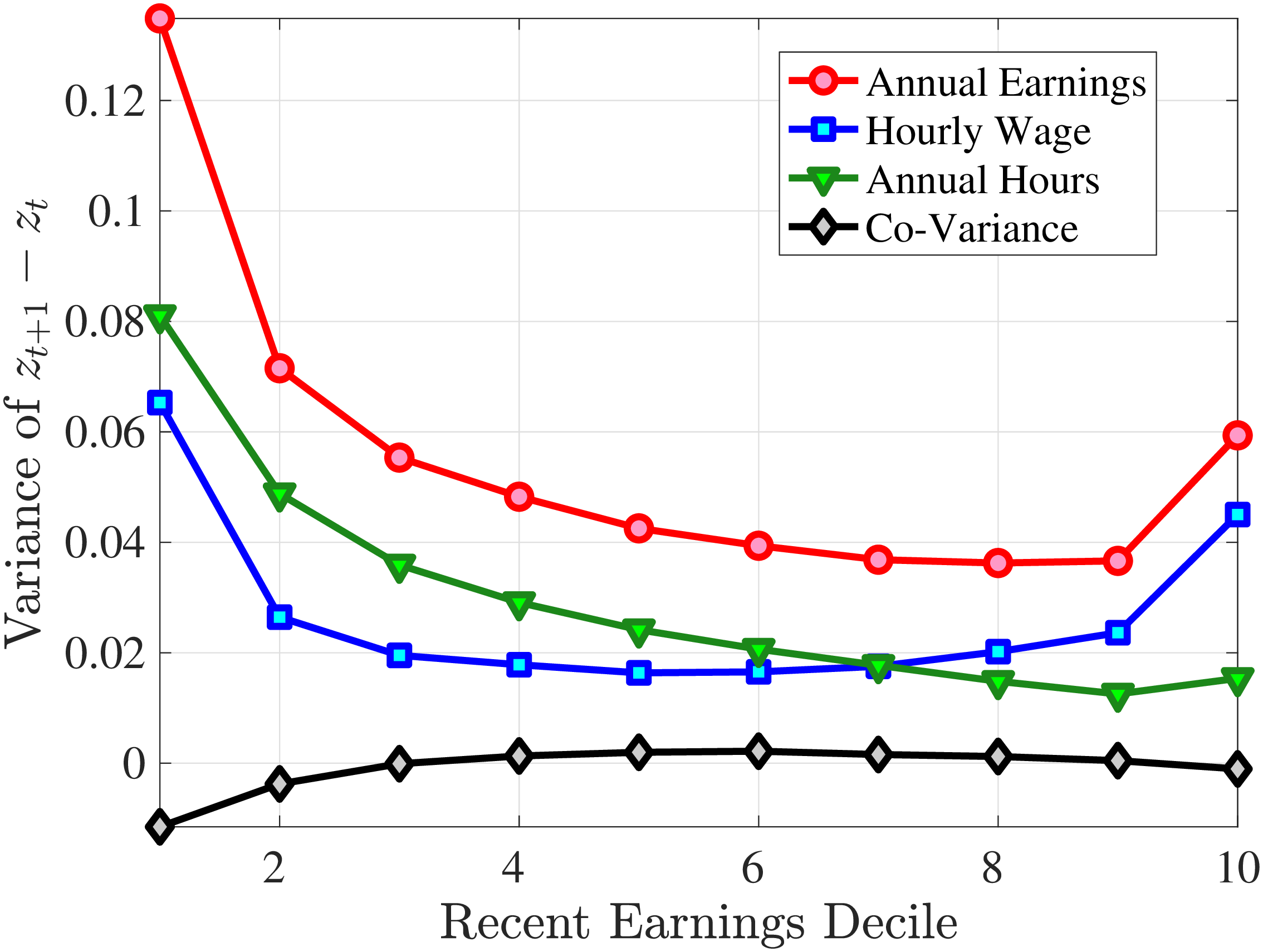(a) Prime-Age Workers: 36–55 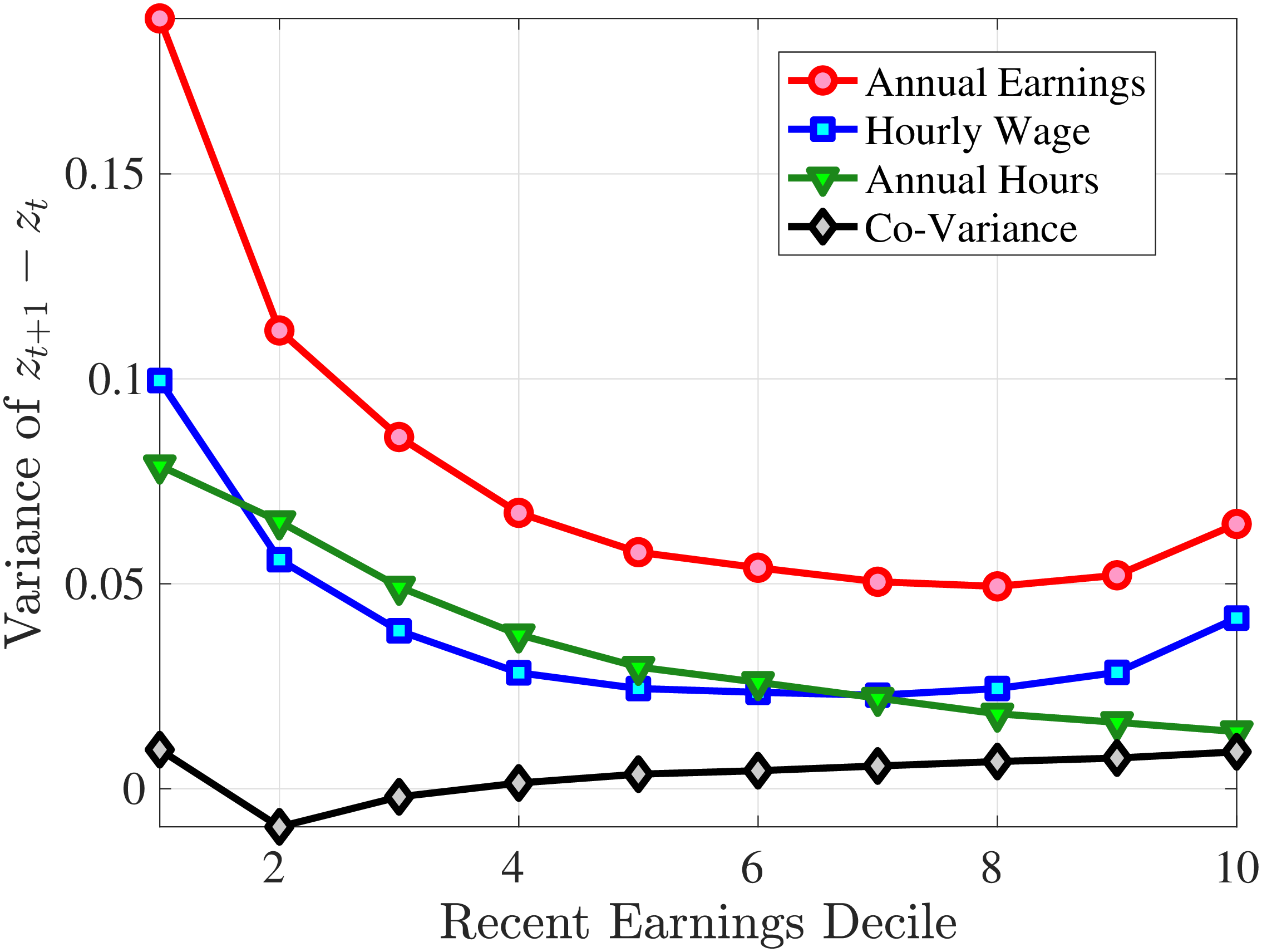(b) Young Workers: 25–35

Figure B.14

–

Decomposition of Variance of One-Year Growth

Note: The figure decomposes the variance of one-year log earnings changes (red line) into the variance of log wage changes (blue line), the variance of log hours changes (green line), and the co-variance between log wage and log hours changes (black line).

Figure: Figure B.14 – Decomposition of Variance of One-Year Growth

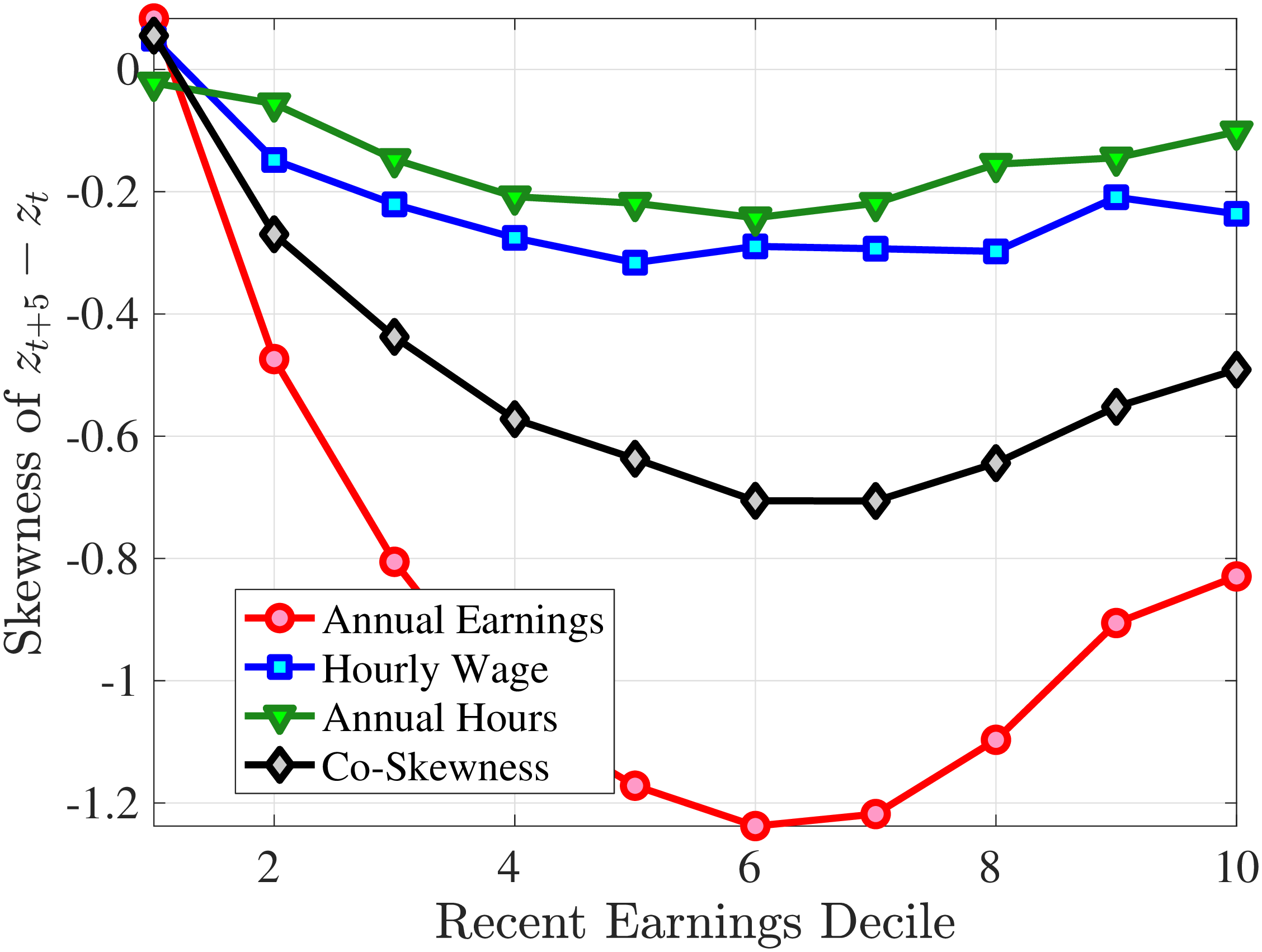
Figure B.15

–

Decomposition of Skewness of Five-Year Growth, Young Workers

Note: The figure decomposes the skewness of five-year log earnings changes (red line) for young workers (ages 25-35) into the skewness of log wage changes (blue line), the skewness of log hours changes (green line), and the co-skewness between log wage and log hours changes (black line). Each dot represents a decile of RE. The decomposition is based on Lemma 1.

Figure: Figure B.15 – Decomposition of Skewness of Five-Year Growth, Young Workers

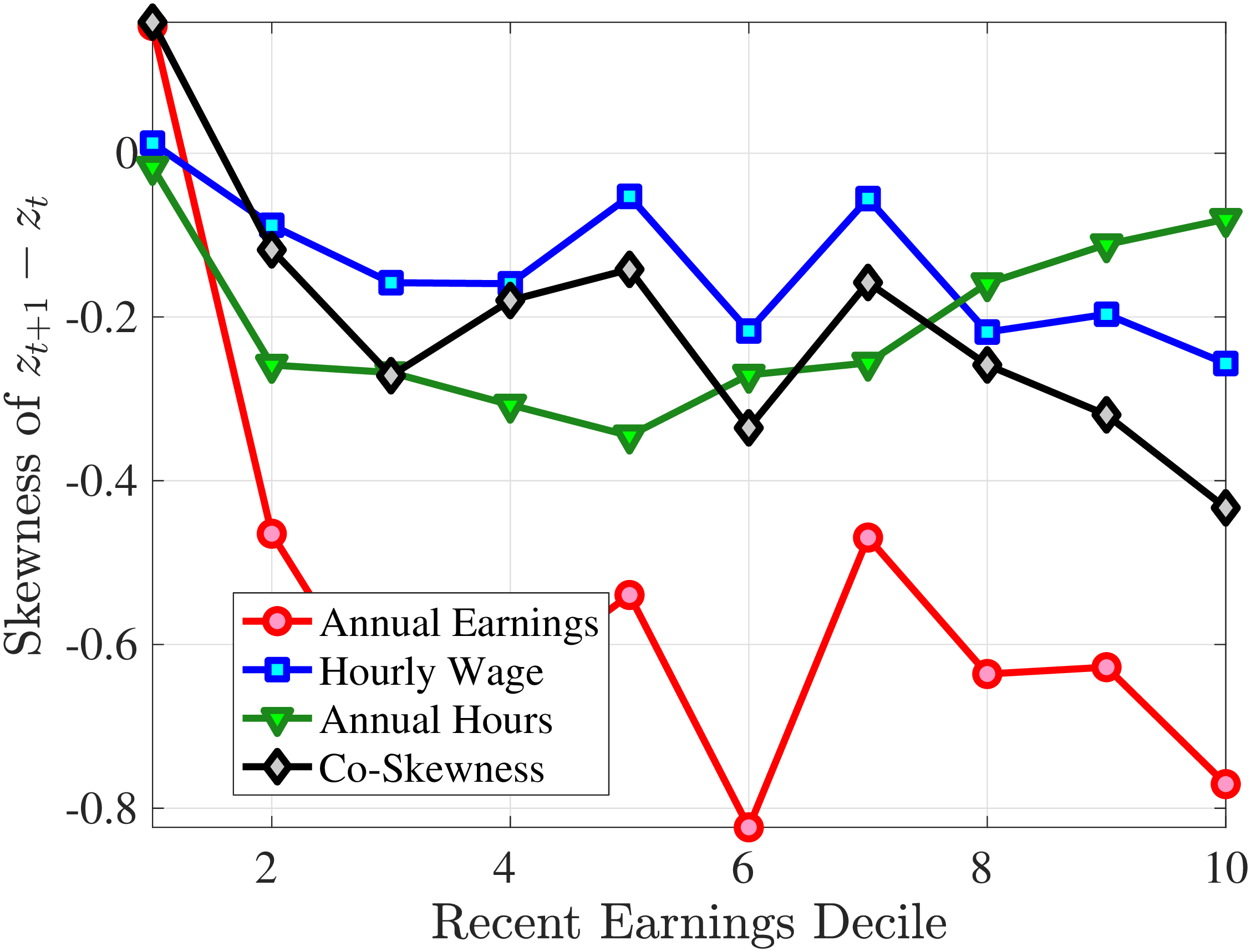(a) Prime-Age Workers: 36–55 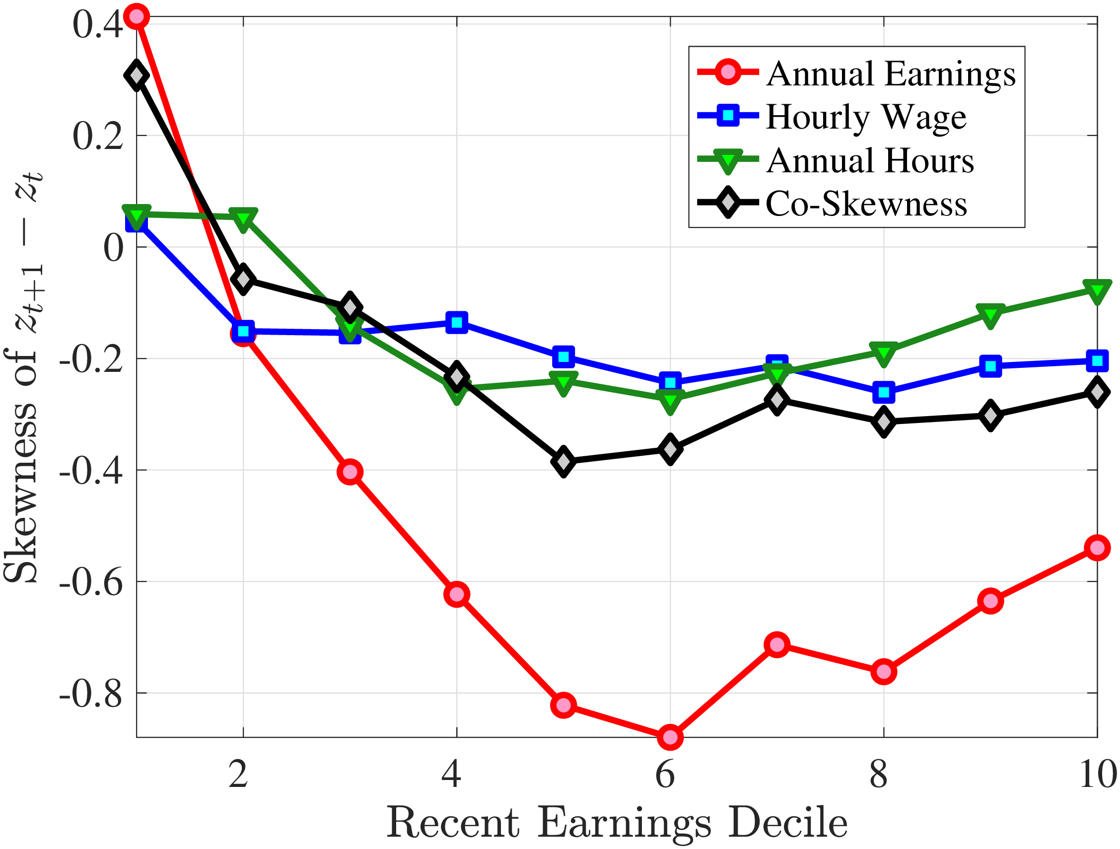(b) Young Workers: 25–35

Figure B.16

–

Decomposition of Skewness of One-Year Growth

Note: The figure decomposes the skewness of one-year log earnings changes (red line) into the skewness of log wage changes (blue line), the skewness of log hours changes (green line), and the co-skewness between log wage and log hours changes (black line). Each dot represents a decile of RE. The decomposition is based on Lemma 1.

Figure: Figure B.16 – Decomposition of Skewness of One-Year Growth

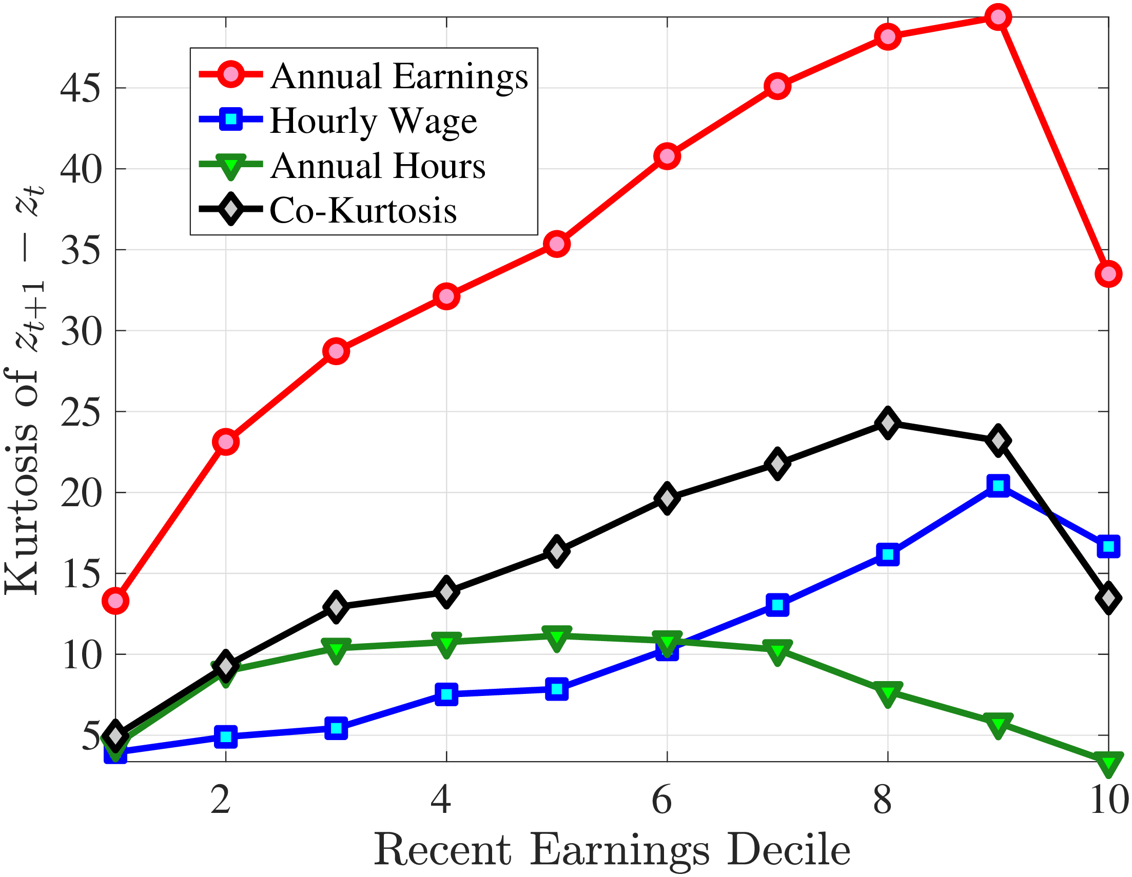(a) Prime-Age Workers: 36–55 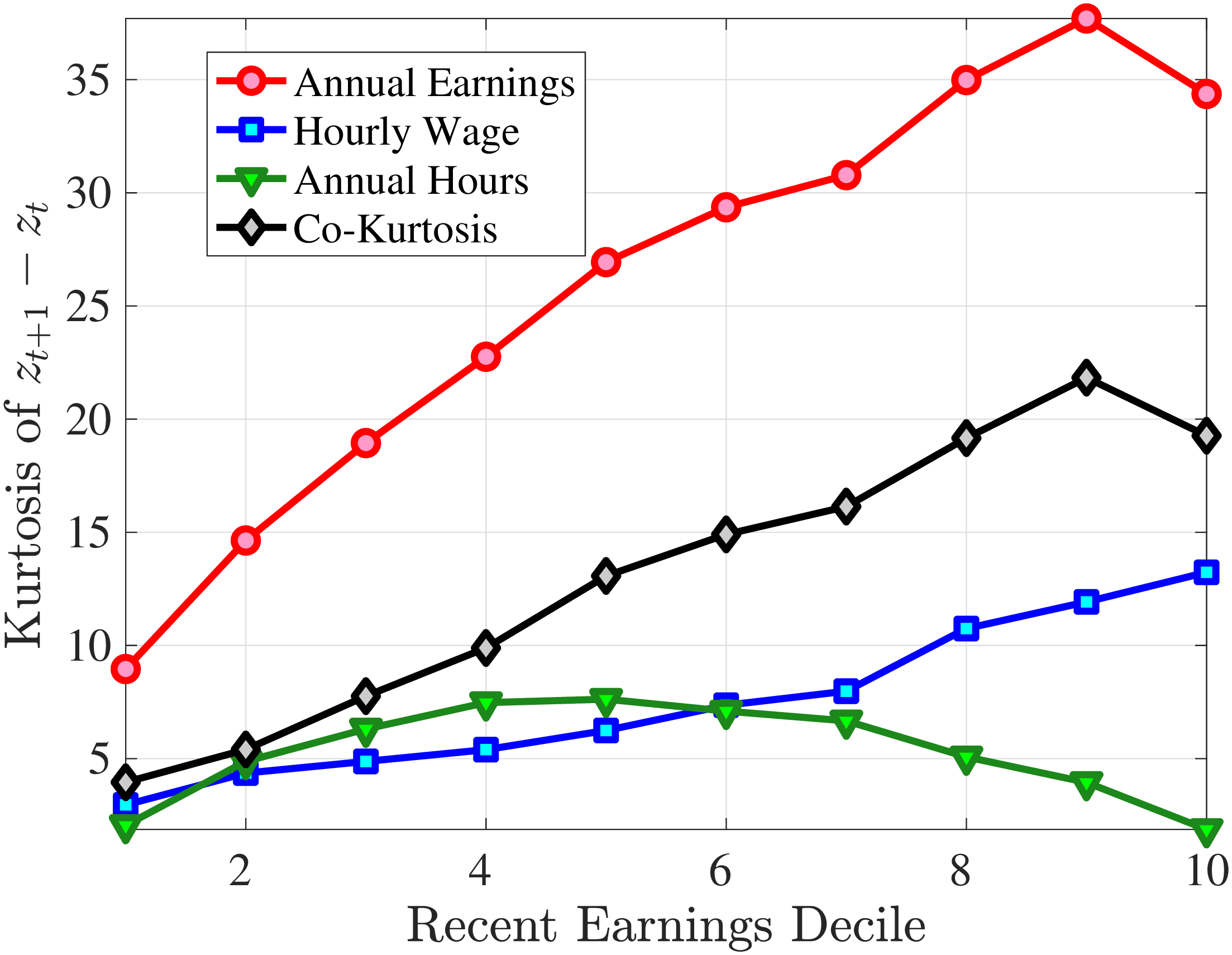(b) Young Workers: 25–35

Figure B.17

–

Decomposition of Kurtosis of One-Year Growth

Note: The figure decomposes the kurtosis of one-year log earnings changes (red line) into the kurtosis of log wage changes (blue line), the kurtosis of log hours changes (green line), and the co-kurtosis between log wage and log hours changes (black line). Each dot represents a decile of RE. The decomposition is based on Lemma 1.

Figure: Figure B.17 – Decomposition of Kurtosis of One-Year Growth

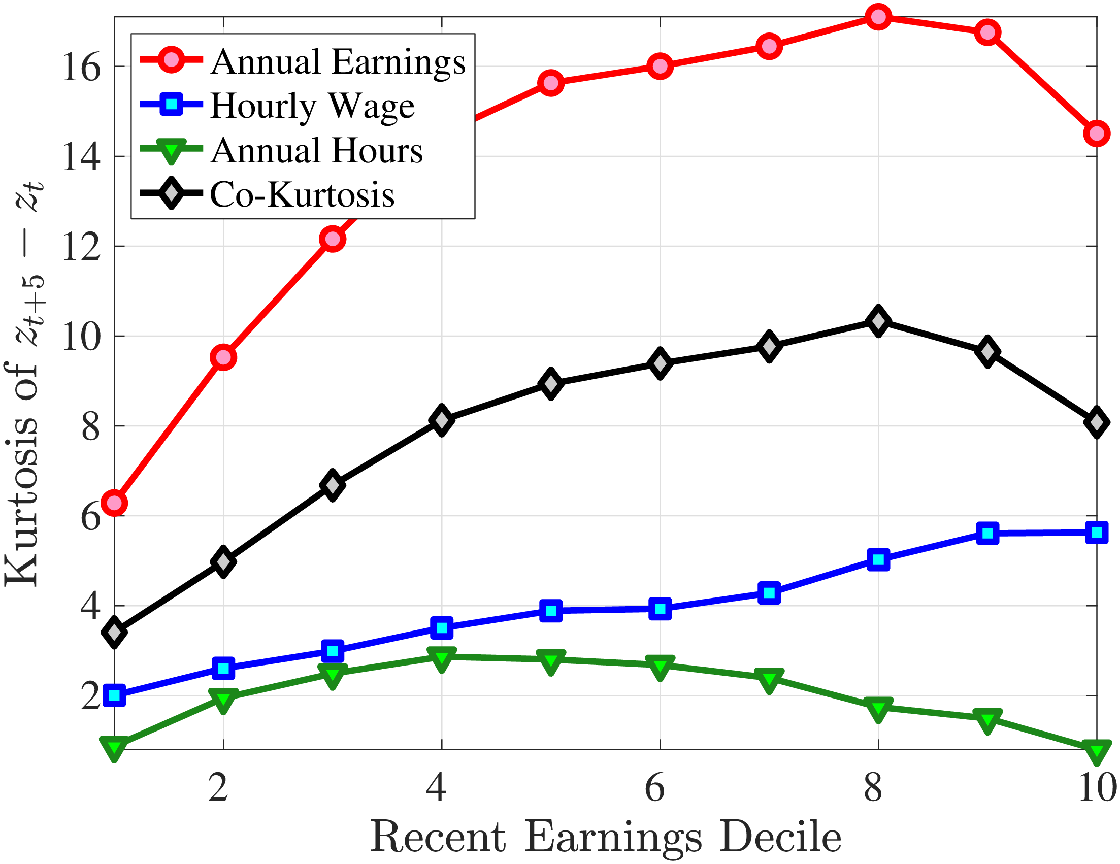
Figure B.18

–

Decomposition of Kurtosis of Five-Year Growth, Young Workers: 25–35

Note: The figure decomposes the kurtosis of five-year log earnings changes (red line) into the kurtosis of log wage changes (blue line), the kurtosis of log hours changes (green line), and the co-kurtosis between log wage and log hours changes (black line). Each dot represents a decile of RE. The decomposition is based on Lemma 1.

Figure: Figure B.18 – Decomposition of Kurtosis of Five-Year Growth, Young Workers: 25–35

8.5 Cross-Sectional Moments of One-Year Growth in Household Earnings and Disposable Income

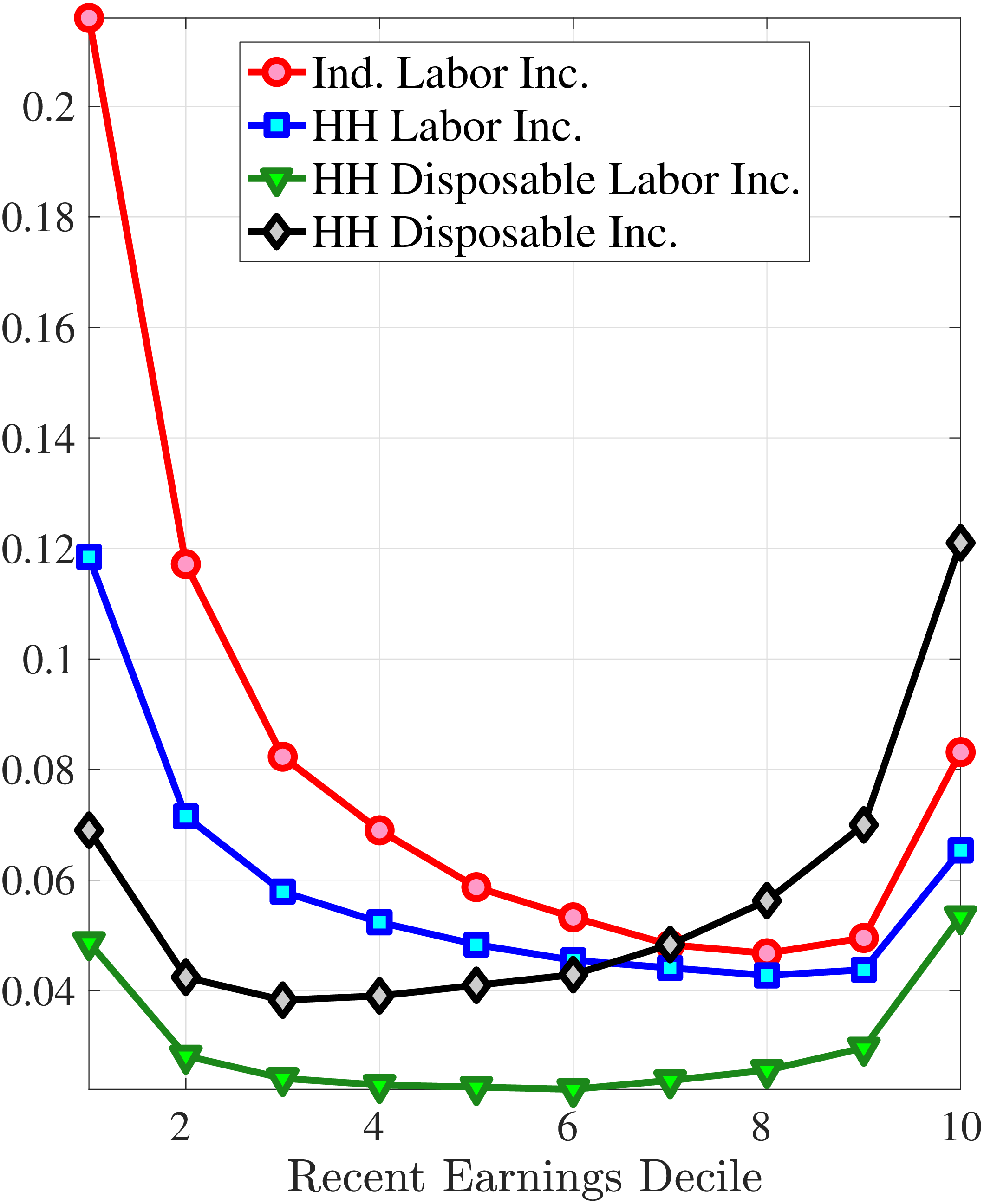(a) Variance of $\Delta _{\log}^{1}y_{t}^{i}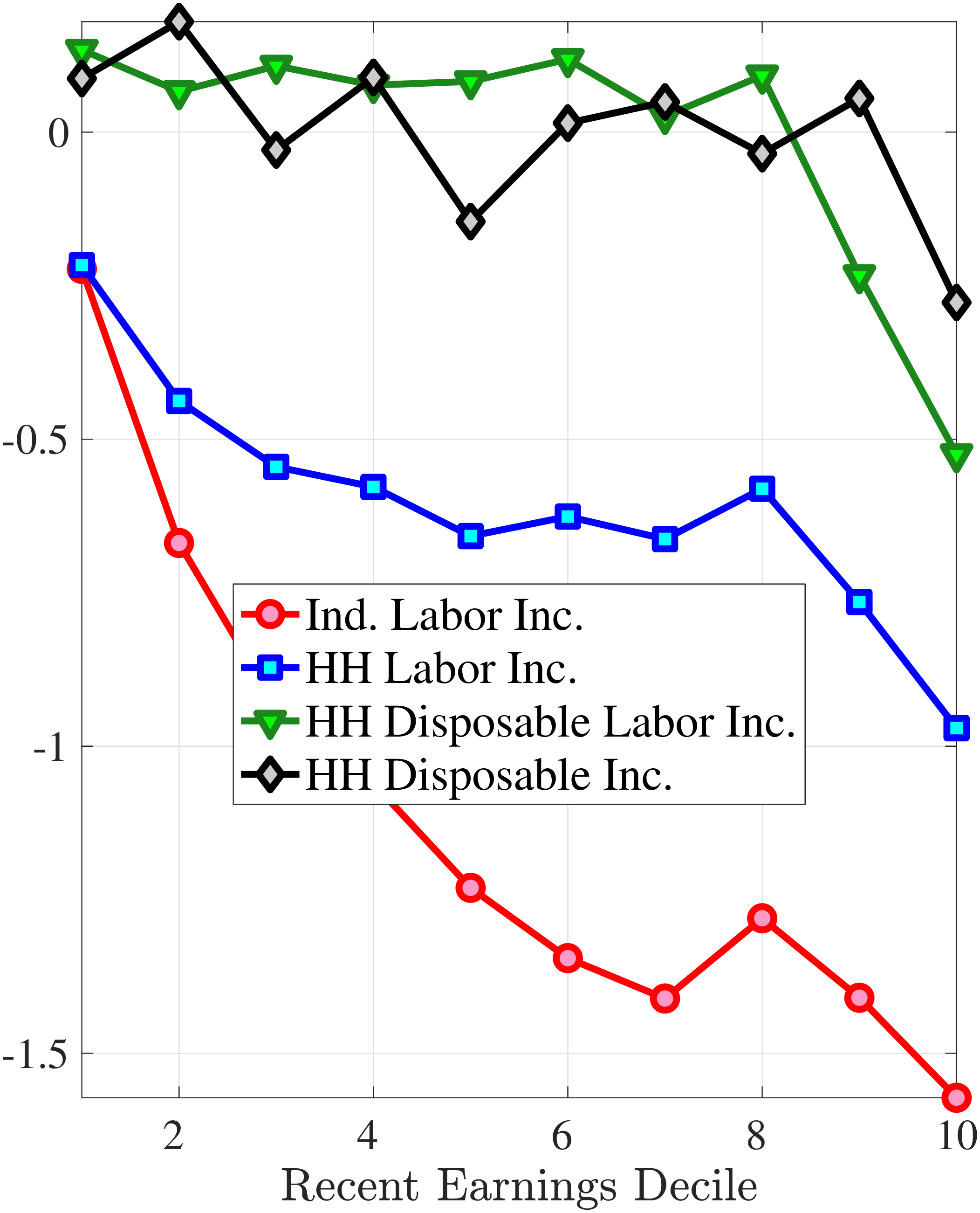$ (b) Skewness of $\Delta _{\log}^{1}y_{t}^{i}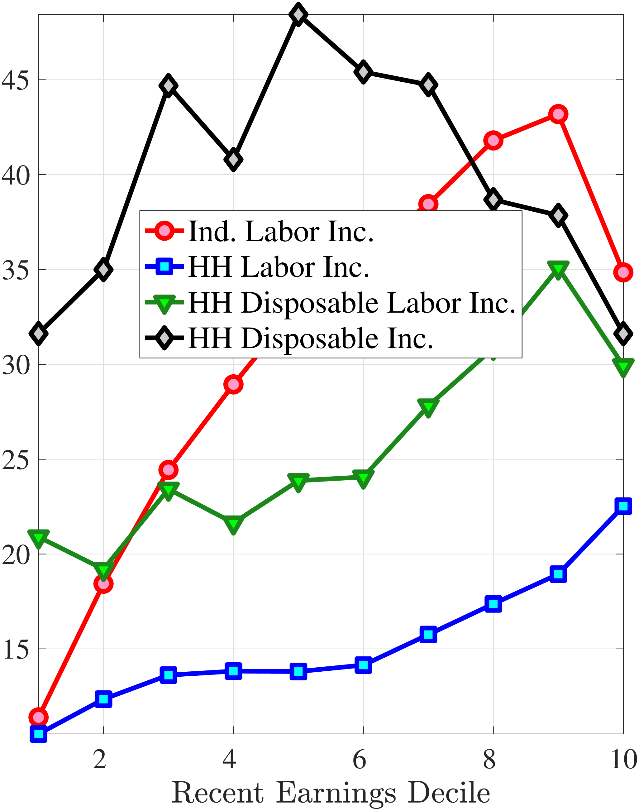$ (c) Kurtosis of $\Delta _{\log}^{1}y_{t}^{i}$

Figure B.19

–

Cross-Sectional Moments of One-Year Log Household Earnings and Disposable Income Growth, Age 36–55

Note:The figure displays the higher-order cross-sectional moments of one-year log earnings changes (red line), log household earnings changes (blue line), log disposable labor income changes (green line), and log disposable income changes (black line) for prime-age males and their households, plotted for each decile of RE. Disposable labor income is defined as disposable income net of after-tax capital income. The sample comprises married and cohabiting men and their households.

Figure: Figure B.19 – Cross-Sectional Moments of One-Year Log Household Earnings and Disposable Income Growth, Age 36–55

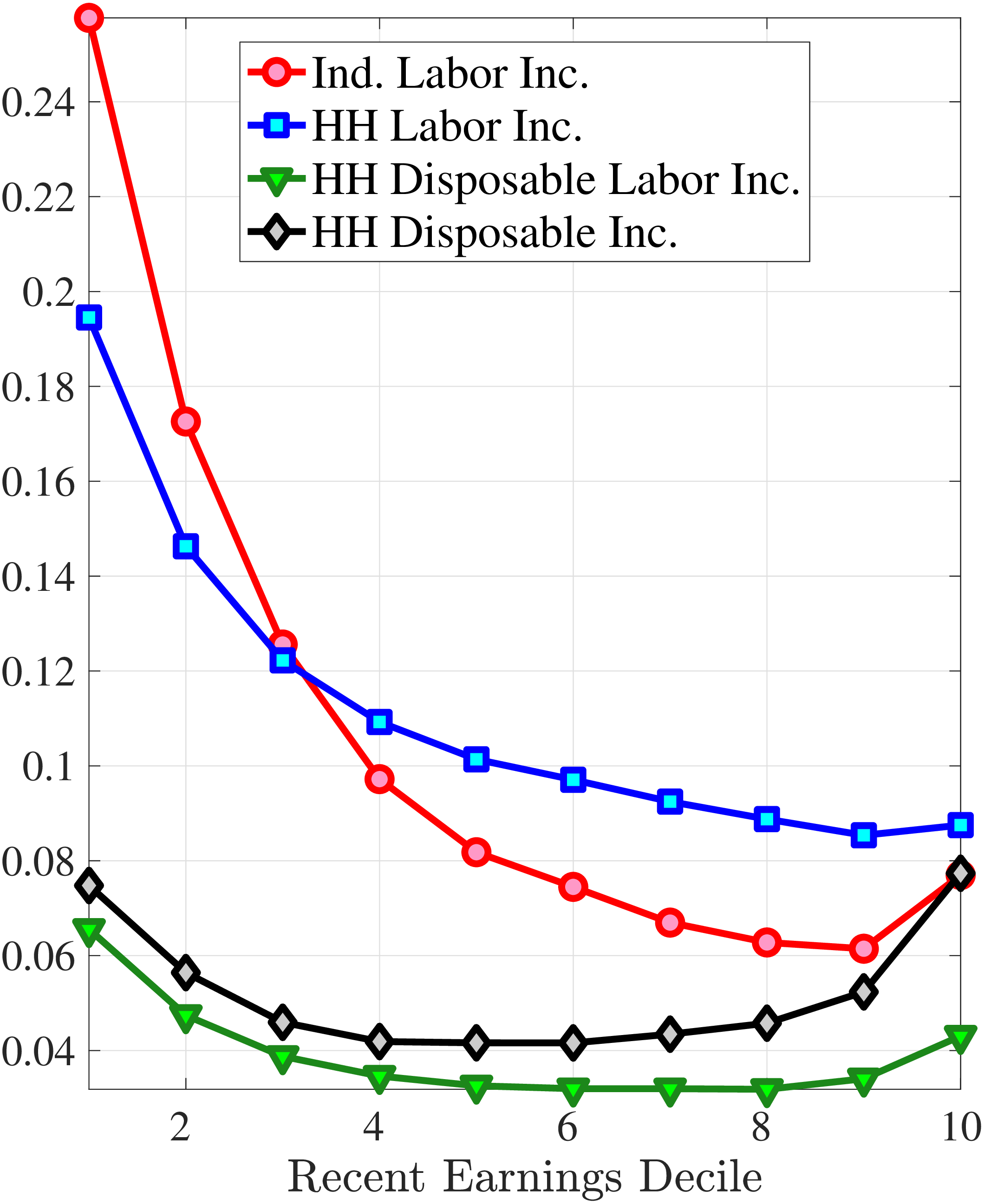(a) Variance of $\Delta _{\log}^{1}y_{t}^{i}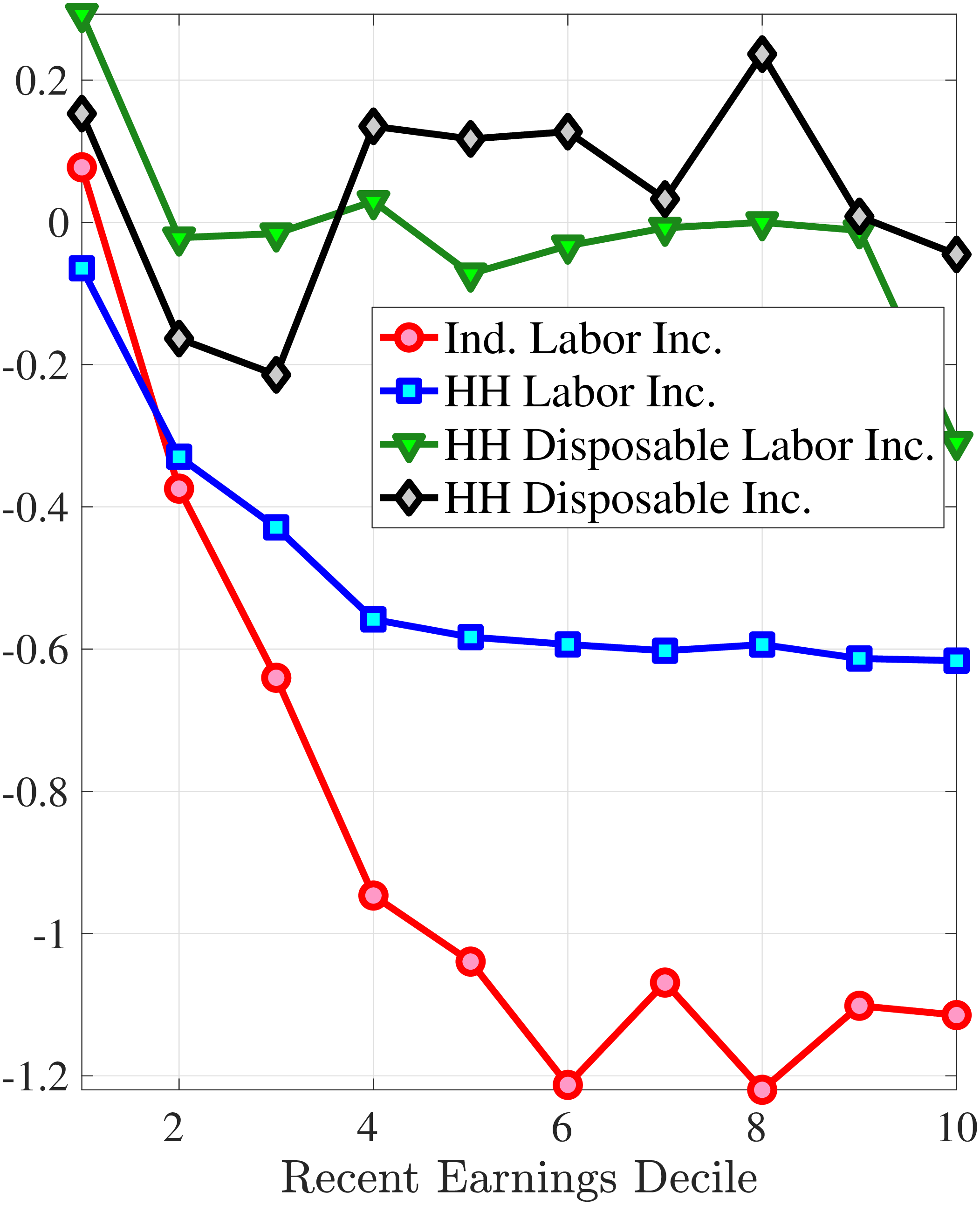$ (b) Skewness of $\Delta _{\log}^{1}y_{t}^{i}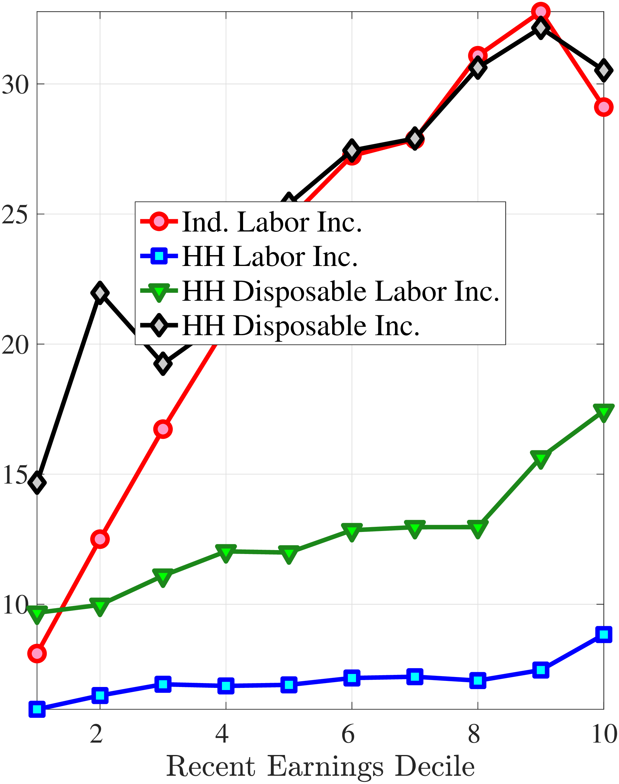$ (c) Kurtosis of $\Delta _{\log}^{1}y_{t}^{i}$

Figure B.20

–

Cross-Sectional Moments of One-Year Log Household Earnings and Disposable Income Growth, Age 25–35

Note: The figure displays the higher-order cross-sectional moments of one-year log earnings changes (red line), log household earnings changes (blue line), log disposable labor income changes (green line), and log disposable income changes (black line) for young males and their households for each decile of RE. Disposable labor income is defined as disposable income net of after-tax capital income. The sample comprises married and cohabiting men and their households.

Figure: Figure B.20 – Cross-Sectional Moments of One-Year Log Household Earnings and Disposable Income Growth, Age 25–35

9 Imputing Hours in the PSID

For comparison with our imputation of hours in the Norwegian data, we obtain data from the Panel Study of Income Dynamics (PSID), 1968-1997. We again employ the regression tree approach to estimate annual hours $h_{it}^{PSID}$ from the PSID using the available variables. The PSID does not contain exactly the same variables as the Norwegian data, but it does contain much of the same information. As in the AKU, we use regression trees of depth 3. At the terminal nodes of the tree (the leaves), we use linear regression models to minimize the errors between the measured and predicted values:⁴²

\[ h_{it}^{PSID}=\beta X_{it}+\epsilon _{it}, \] where $X_{it}$ contains demographic information such as marital status and number of sickness days. As in the AKU, we perform the imputation exercise both including and not including labor earnings (wage) as an explanatory variable. Figures C.1 and C.2 display the regression trees for men and women when labor earnings is used as an explanatory variable and Figures C.3 and C.4 display the regression trees when labor earnings is not included as a regressor. Table C.1 displays the $R$-squared in the training and test samples for men and women when we include or exclude labor earnings as an explanatory variable. We observe that the explanatory power (as measured by the $R$-squared) of our variables in PSID, as in the Norwegian register data, is greater for women than for men. It also matters significantly for the $R$-squared whether we include annual earnings as an explanatory variable. Including annual earnings plays an even larger role in the PSID than in the Norwegian data. The training sample $R$-squareds are as high as 49% for men and 69% for women when labor earnings is included and only 18% for men and 28% for women when labor earnings is not included.

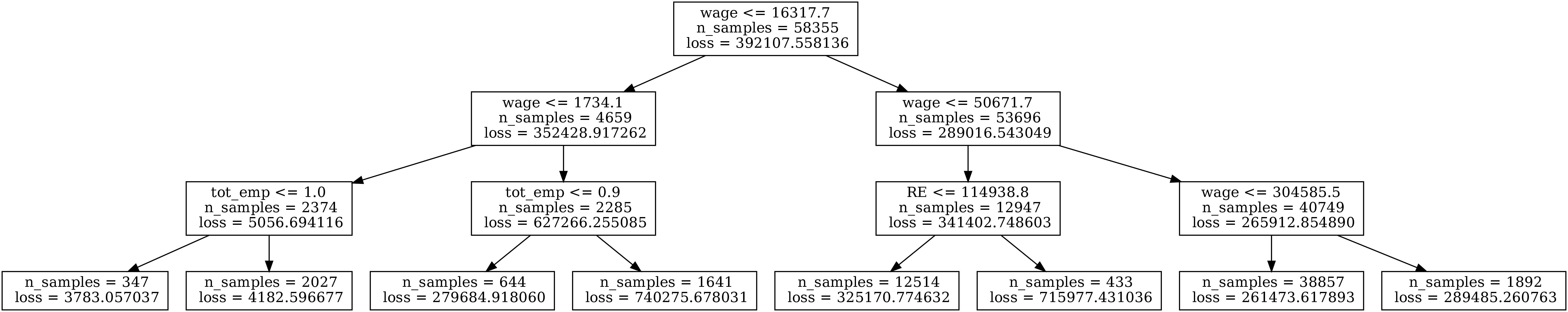
Figure: Figure C.1 – Regression Tree Structure for Men in the PSID

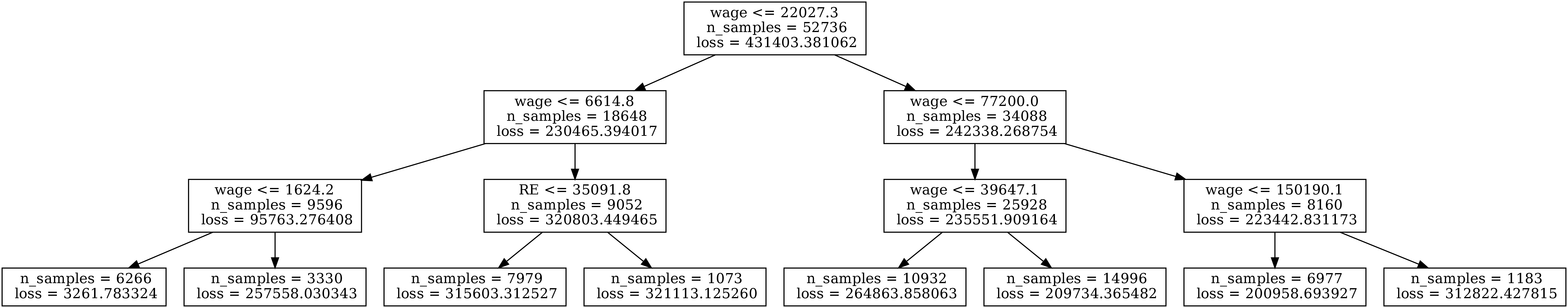
Figure: Figure C.2 – Regression Tree Structure for Women in the PSID

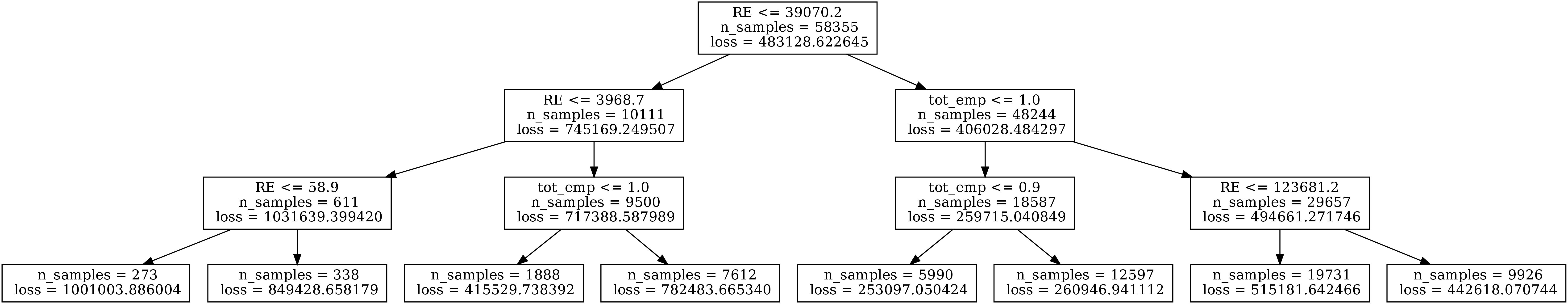
Figure: Figure C.3 – Regression Tree Structure for Men in the PSID without Earnings

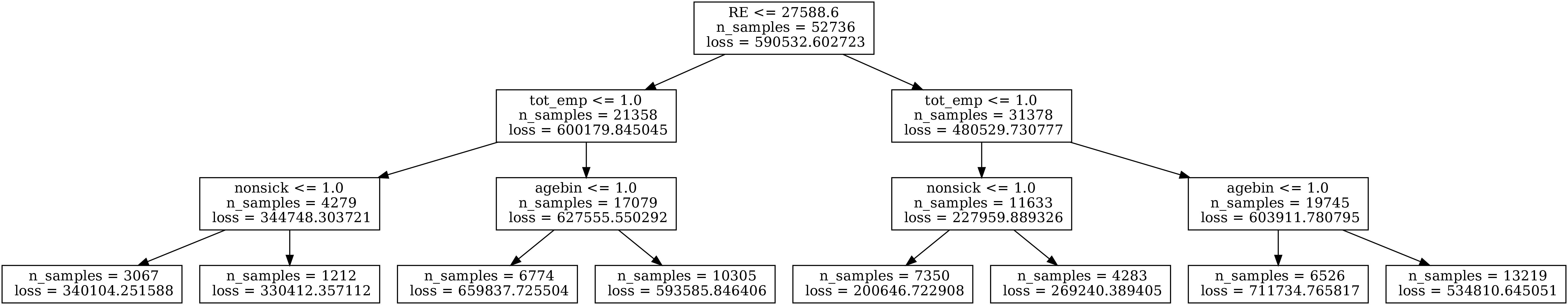
Figure: Figure C.4 – Regression Tree Structure for Women in the PSID without Earnings

	Level
Depth	3	3
Wage	Yes	No
Men	49.43	18.25
Test	51.66	17.79
Women	68.55	28.21
Test	68.20	28.08

Table C.1 – $R^{2}$ of Selected Regression Tree Models for the PSID

Note:

The dependent variable is the level of hours and the independent variables are annual earnings, the fraction of non-sick

days, non-unemployment days, and days employed. We also include the arc-percent changes of these variables between

$t$

and

$t-1$

Furthermore, an indicator variable for marital status and its change from last year (

$t-1$

) are included. Finally, we control for recent

earnings, age, and education of the worker.

10 Additional Results for Men

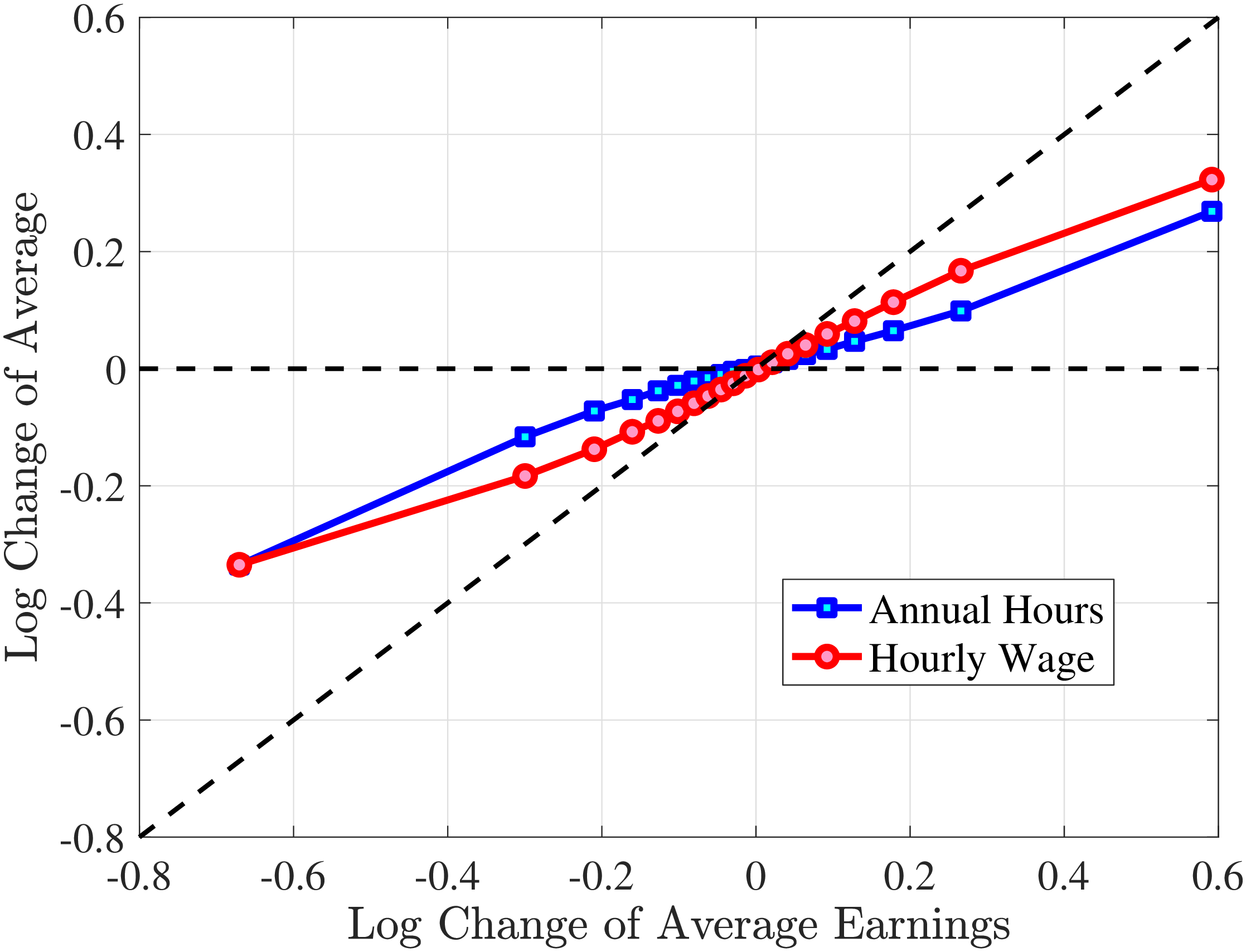
Figure D.1

–

Contributions of Hours and Wage Rates to Earnings Shocks for 4th-7th RE Deciles (Young Men)

Note: The figure displays the one-year Representative-Agent change (i.e., log change of averages) for imputed hours and imputed wage rates for 20 different groups of young males (ages 25–35) in the 4th-7th RE deciles, plotted against their contemporaneous one-year log change in average annual earnings.

Figure: Figure D.1 – Contributions of Hours and Wage Rates to Earnings Shocks for 4th-7th RE Deciles (Young Men)

1st RE Decile

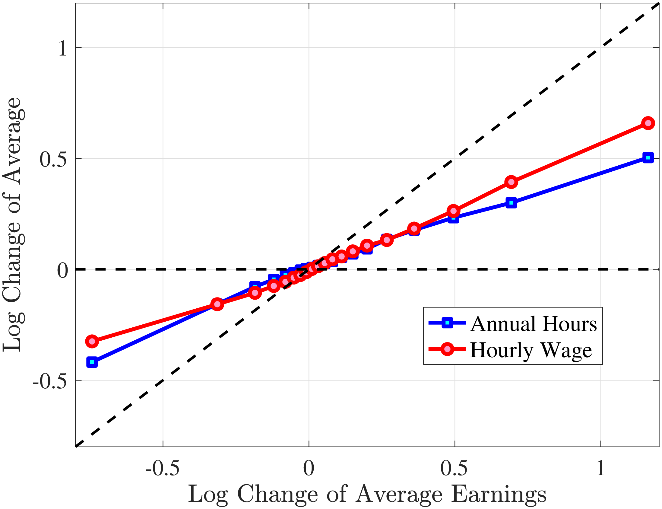
10th RE Decile

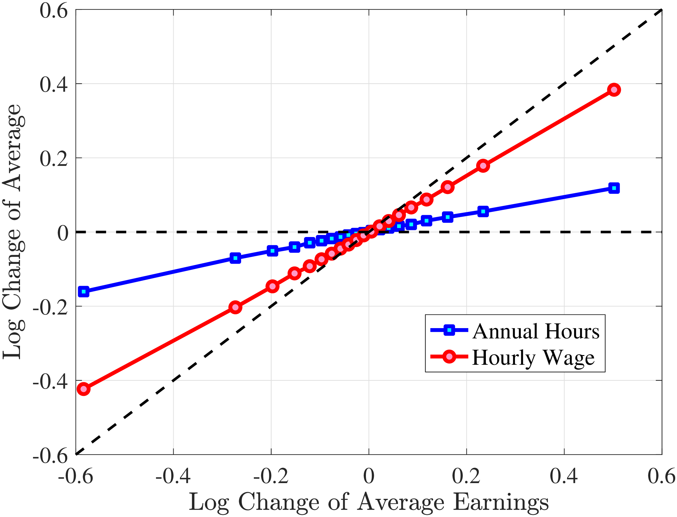
Figure D.2

–

Contributions of Hours and Wage Rates to Earnings Shocks (Young Men)

Note: The figure displays the one-year Representative-Agent change (i.e., log change of averages) for imputed hours and imputed wage rates for 20 different groups of young males (ages 25–35) in the 1st and 10th RE deciles, plotted against their contemporaneous one-year log change in average annual earnings.

Figure: Figure D.2 – Contributions of Hours and Wage Rates to Earnings Shocks (Young Men)

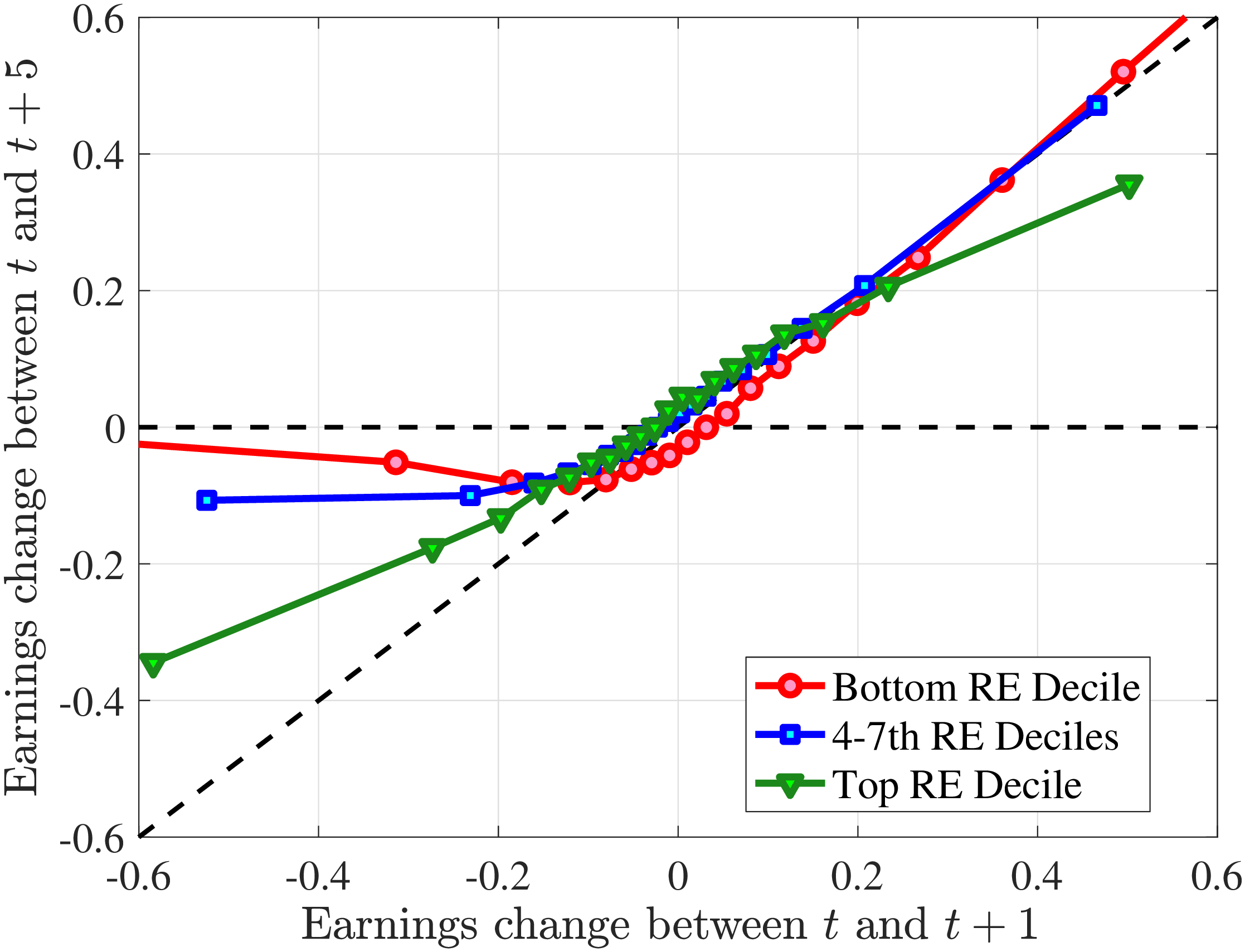
Figure D.3

–

Persistence of Earnings Changes, Young Males

Note: The figure displays the five-year Representative-Agent change (i.e., log change of averages) in earnings for 20 different groups of young males (ages 25–35) in the 1st RE decile (red line), 4th-7th RE deciles (blue line), and 10th RE decile (green line), plotted against their respective one-year log change in average annual earnings.

Figure: Figure D.3 – Persistence of Earnings Changes, Young Males

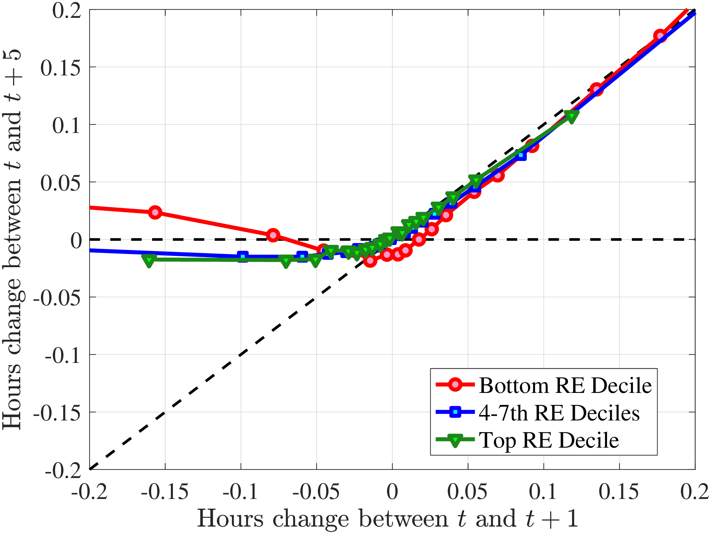(a) Annual Hours 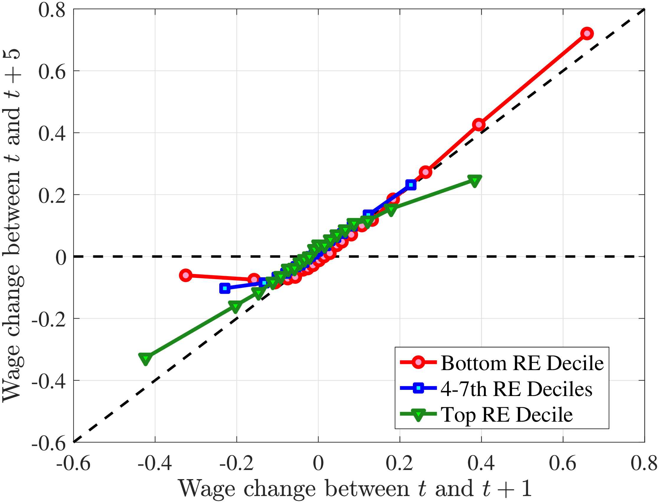(b) Hourly Wage

Figure D.4

–

Persistence of Hours and Hourly Wage Changes by RE Decile, Young Males

Note: The left panel displays the five-year Representative-Agent change (i.e., log change of averages) in imputed annual hours for 20 different groups of young males (ages 25–35) in the 1st RE decile (red line), 4th-7th RE deciles (blue line), and 10th RE decile (green line), plotted against their respective one-year log change in imputed annual average hours. The right panel displays the corresponding figure for imputed hourly wage rates.

Figure: Figure D.4 – Persistence of Hours and Hourly Wage Changes by RE Decile, Young Males

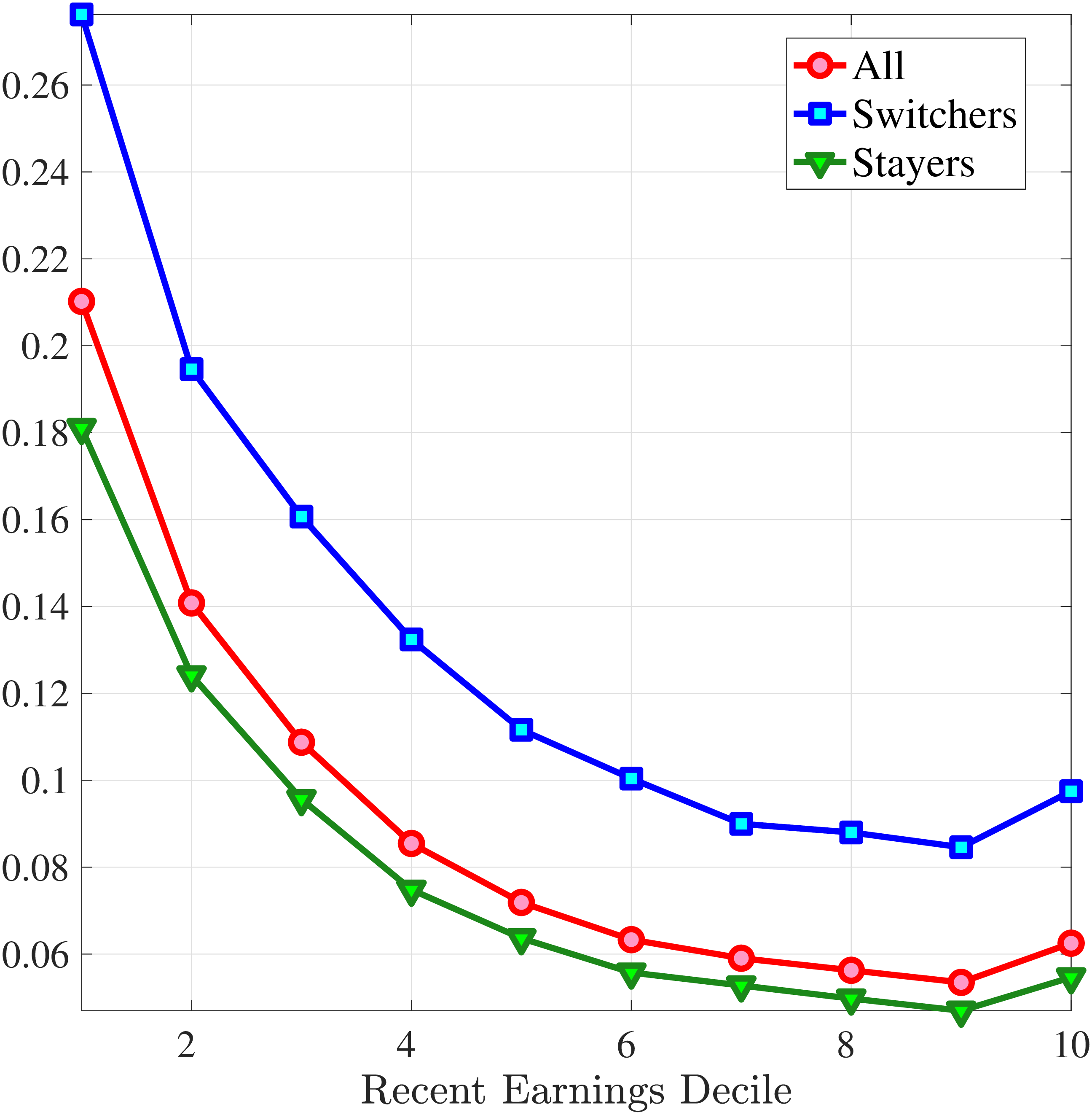(a) Variance of $\Delta _{\log}^{1}y_{t}^{i}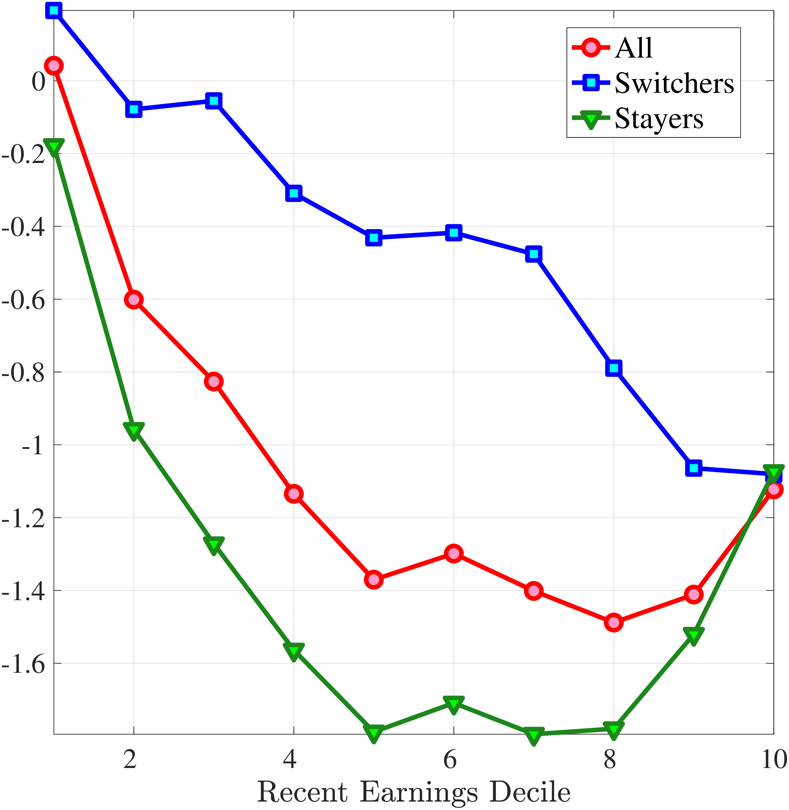$ (b) Skewness of $\Delta _{\log}^{1}y_{t}^{i}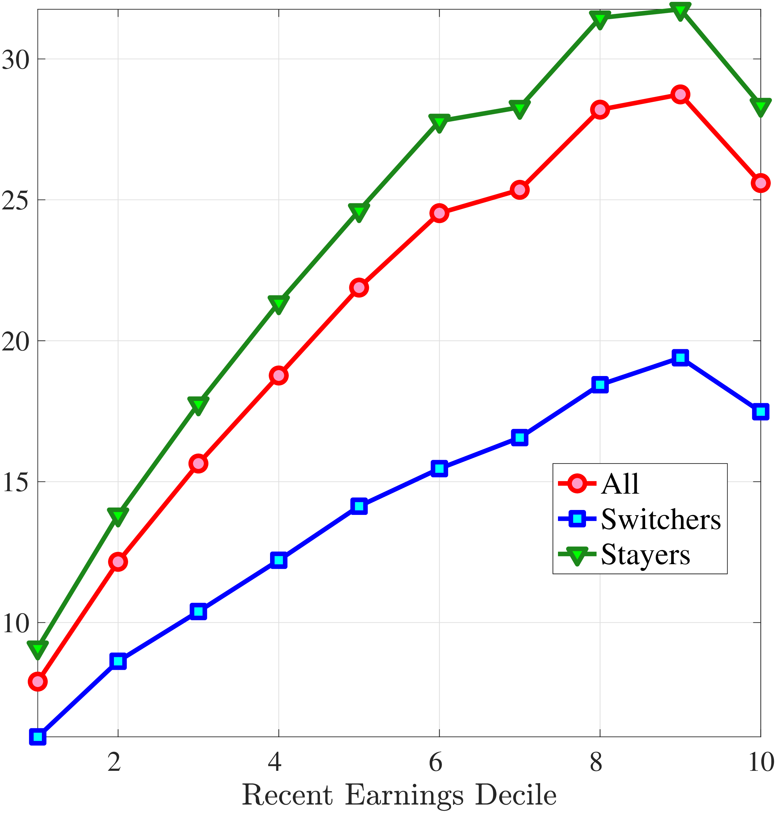$ (c) Kurtosis of $\Delta _{\log}^{1}y_{t}^{i}$

Figure D.5

–

Cross-Sectional Moments of One-Year Log Earnings Growth (Young Males): Stayers vs. Switchers ($y_{t+1}-y_{t}$)

Note: The figure displays the higher-order moments of log earnings growth for job switchers (blue line), job stayers (green line), and all young males (red line) for each RE decile.

Figure: Figure D.5 – Cross-Sectional Moments of One-Year Log Earnings Growth (Young Males): Stayers vs. Switchers ($y_{t+1}-y_{t}$)

Skewness

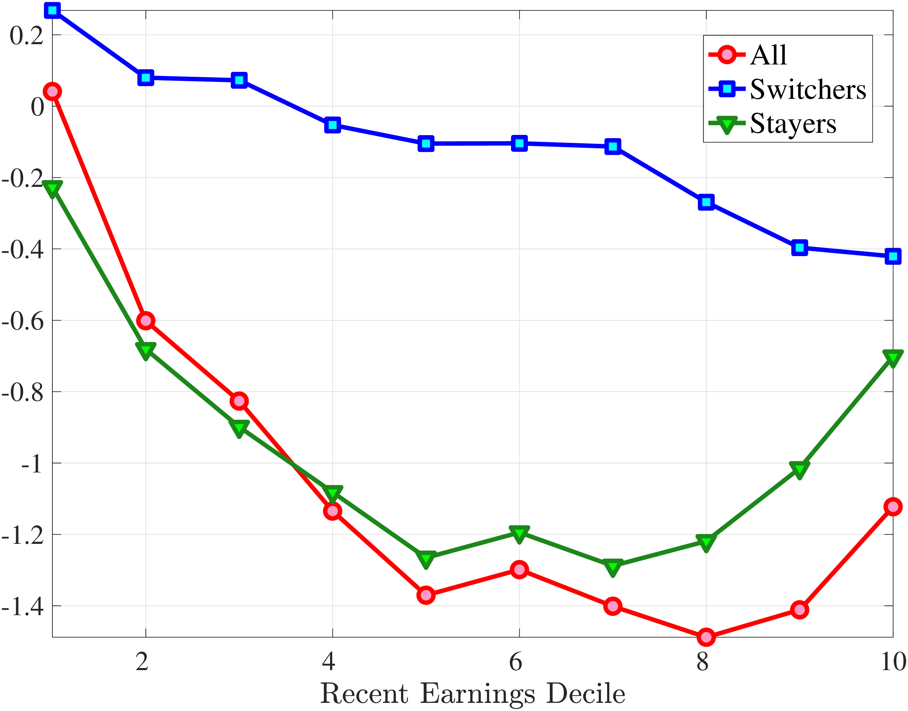
Kurtosis

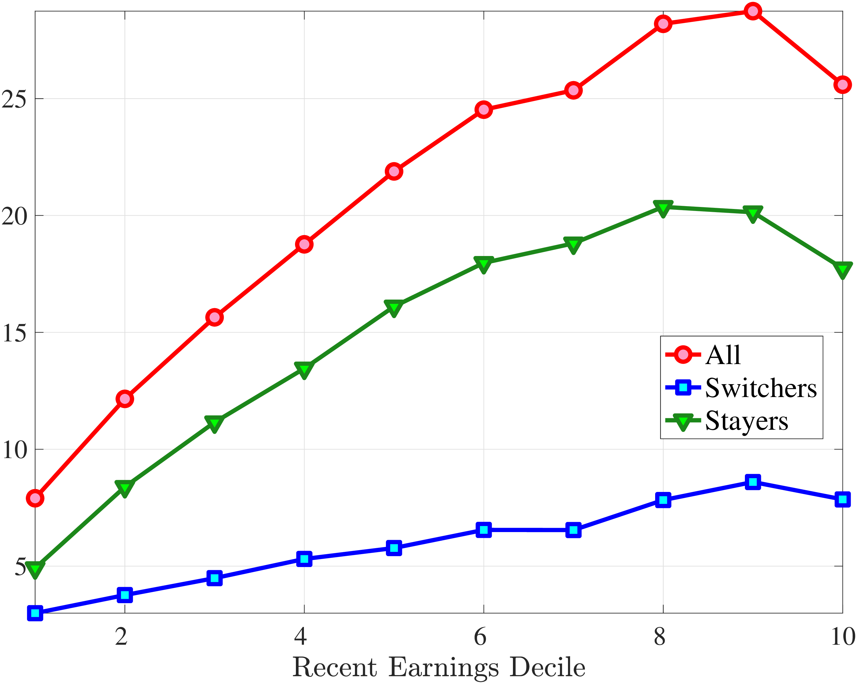
Figure D.6

–

Contribution of Job Stayers and Job Switchers to Skewness and Kurtosis of Earnings Growth (Young Males)

Note: The figure displays the contributions of job switchers (blue line) and job stayers (green line) to the population skewness and kurtosis of one-year earnings growth for young males (red line) for each RE decile.

Figure: Figure D.6 – Contribution of Job Stayers and Job Switchers to Skewness and Kurtosis of Earnings Growth (Young Males)

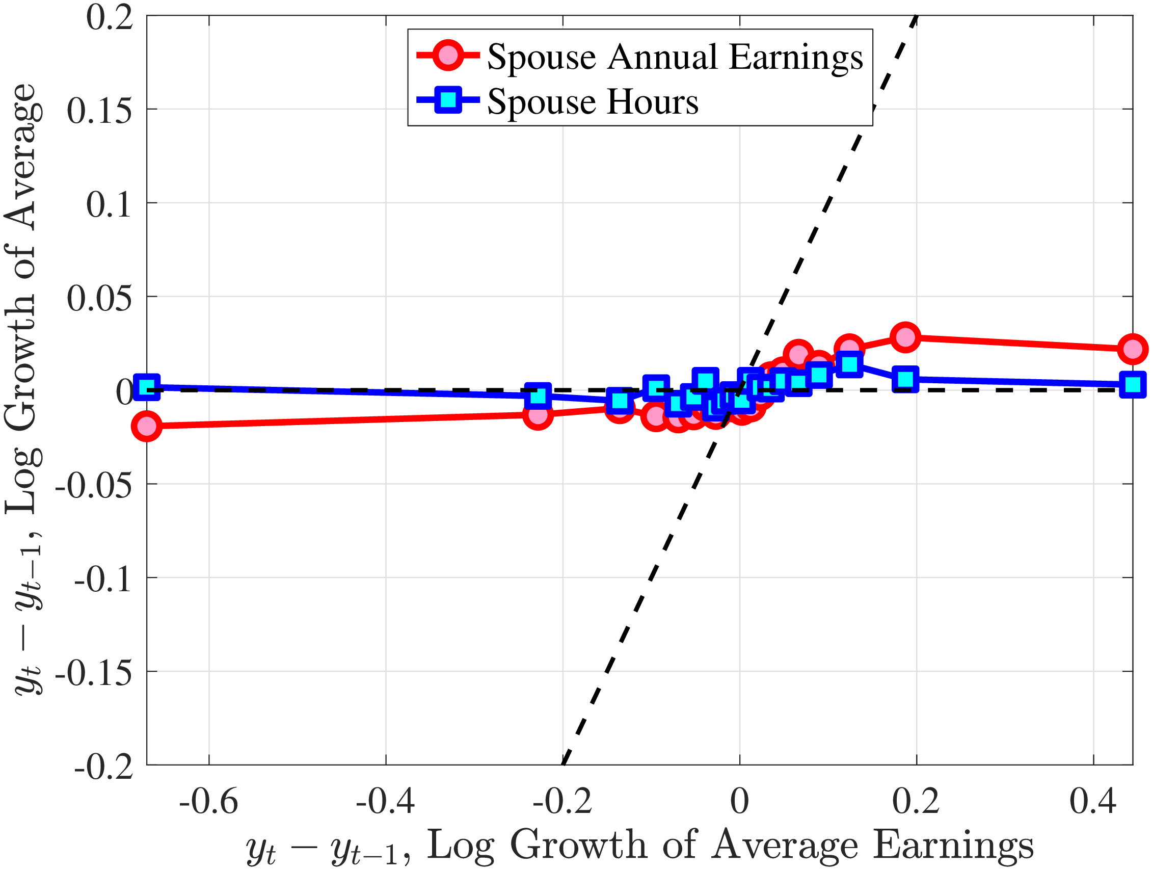
Figure D.7

–

Spousal Responses to Male Earnings Shocks

Note: The figure displays the one-year Representative-Agent change (i.e., log change of averages) of spousal annual earnings and imputed hours for 20 different groups of prime-age males (ages 36–55), plotted against their contemporaneous one-year log change in average annual earnings. The sample comprises men and women who are married or cohabiting.

Figure: Figure D.7 – Spousal Responses to Male Earnings Shocks

Table D.1 displays the fraction of male workers with large and small, and positive and negative five-year earnings changes that experience certain events.

					Five year Earnings Change, $\Delta _{\log}^{5}y_{t}^{i}\in$
All		Five-Year Earnings Loss			Five-Year Earnings Gain
Life-cycle event in $t+1$		$\lt -0.5$	$[-0.5,-0.25)$	$[-0.25,0.0)$	$[0.0,0.25)$	$[0.25,0.5)$	$\geq 0.5$
into/out of		(1)	(2)	(3)	(4)	(5)	(6)
(1)	Unemployment	0.02	0.02	0.01	0.01	0.03	0.05
(2)	Long-term sickness	0.10	0.08	0.06	0.06	0.10	0.12
(3)	Part-time	0.09	0.09	0.07	0.09	0.14	0.17
(4)	Parental leave	0.03	0.04	0.04	0.04	0.07	0.06
(5)	Firm change	0.16	0.16	0.12	0.13	0.22	0.26
(6)	$\mathbb{E}\left [\Delta _{\log}^{1}h_{t}^{i}\right]$	-0.06	-0.05	-0.02	0.00	0.10	0.21
(7)	$\mathbb{E}\left [\Delta _{\log}^{5}h_{t}^{i}\right]$	-0.43	-0.23	-0.02	0.03	0.19	0.34
(8)	$\mathbb{E}\left [\Delta _{\log}^{1}w_{t}^{i}\right]$	-0.06	-0.05	-0.01	0.01	0.11	0.21
(9)	$\mathbb{E}\left [\Delta _{\log}^{5}w_{t}^{i}\right]$	-0.49	-0.33	-0.07	0.06	0.33	0.53
(10)	# of Obs.	144,461	370,678	984,426	1,041,770	398,811	140,775
Lowest decile (RE=1)		(1)	(2)	(3)	(4)	(5)	(6)
(1)	Unemployment	0.04	0.04	0.03	0.03	0.06	0.05
(2)	Long-term sickness	0.10	0.08	0.06	0.05	0.06	0.07
(3)	Part-time	0.08	0.08	0.07	0.15	0.21	0.23
(4)	Parental leave	0.02	0.03	0.03	0.03	0.03	0.02
(5)	Firm change	0.18	0.17	0.16	0.19	0.26	0.32
(6)	$\mathbb{E}\left [\Delta _{\log}^{1}h_{t}^{i}\right]$	-0.06	-0.04	-0.03	-0.00	0.06	0.21
(7)	$\mathbb{E}\left [\Delta _{\log}^{5}h_{t}^{i}\right]$	-0.46	-0.16	-0.04	0.03	0.15	0.36
(8)	$\mathbb{E}\left [\Delta _{\log}^{1}w_{t}^{i}\right]$	-0.05	-0.02	-0.00	0.02	0.06	0.26
(9)	$\mathbb{E}\left [\Delta _{\log}^{5}w_{t}^{i}\right]$	-0.49	-0.18	-0.05	0.07	0.20	0.61
(10)	# of Obs.	13,532	13,043	38,560	47,966	23,684	30,040
Top decile (RE=10)		(1)	(2)	(3)	(4)	(5)	(6)
(1)	Unemployment	0.01	0.01	0.00	0.00	0.01	0.02
(2)	Long-term sickness	0.04	0.04	0.03	0.03	0.04	0.04
(3)	Part-time	0.13	0.11	0.08	0.09	0.10	0.14
(4)	Parental leave	0.03	0.04	0.03	0.04	0.06	0.06
(5)	Firm change	0.20	0.18	0.14	0.13	0.16	0.19
(6)	$\mathbb{E}\left [\Delta _{\log}^{1}h_{t}^{i}\right]$	-0.05	-0.03	-0.01	0.01	0.02	0.07
(7)	$\mathbb{E}\left [\Delta _{\log}^{5}h_{t}^{i}\right]$	-0.20	-0.06	-0.01	0.04	0.09	0.15
(8)	$\mathbb{E}\left [\Delta _{\log}^{1}w_{t}^{i}\right]$	-0.16	-0.07	-0.02	0.02	0.06	0.15
(9)	$\mathbb{E}\left [\Delta _{\log}^{5}w_{t}^{i}\right]$	-0.69	-0.28	-0.09	0.05	0.25	0.62
(10)	# of Obs.	16,775	26,355	87,884	88,004	25,967	11,586

Table D.1 – Important Life Cycle Events Associated with 5-Year Earnings Changes

10.1 Decomposing Earnings Shocks Into Hours and Wage Shocks Using Actual AKU Hours Data and Register Hours Data

Figure D.8 – Contribution of Hours and Wages to Male Earnings Shocks, 3rd RE Quintile (AKU Hours Data)

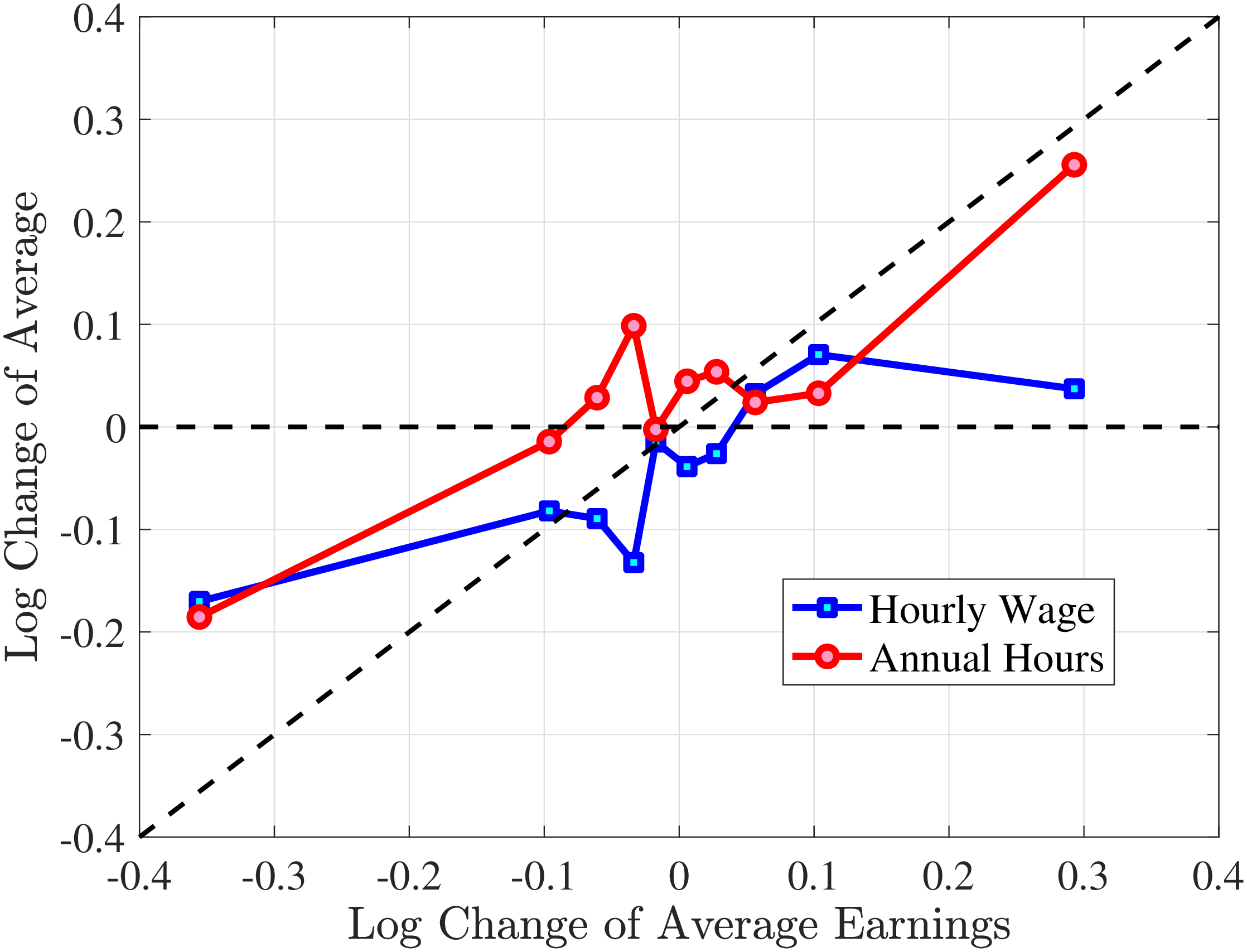
1st RE Quintile

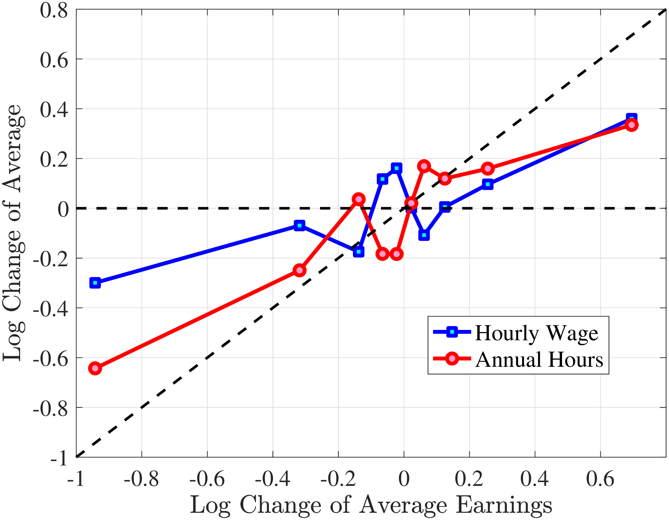
5th RE Quintile

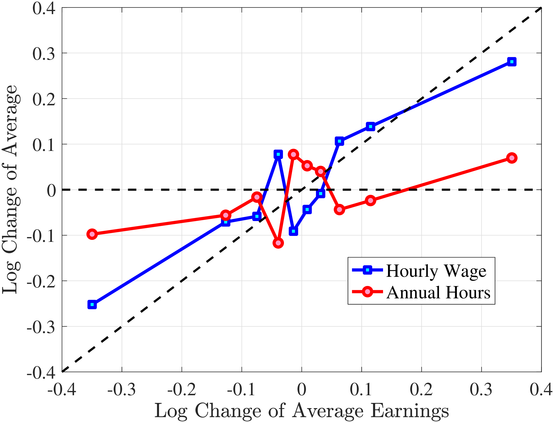
Figure D.9

–

Contribution of Hours and Wage Rates to Male Earnings Shocks (AKU Hours Data)

Note: The figure displays the one-year Representative-Agent change (i.e., log change of averages) for imputed hours and imputed wage rates for 10 different groups of prime-age males (ages 36–55) in the 1st RE quintile (left panel) and 5th RE quintile (right panel), plotted against their contemporaneous one-year log change in average annual earnings.

Figure: Figure D.9 – Contribution of Hours and Wage Rates to Male Earnings Shocks (AKU Hours Data)

Figure D.10 – Contribution of Hours and Hourly Wages to Male Earnings Shocks, 4th-7th RE Deciles (Register Hours Data)

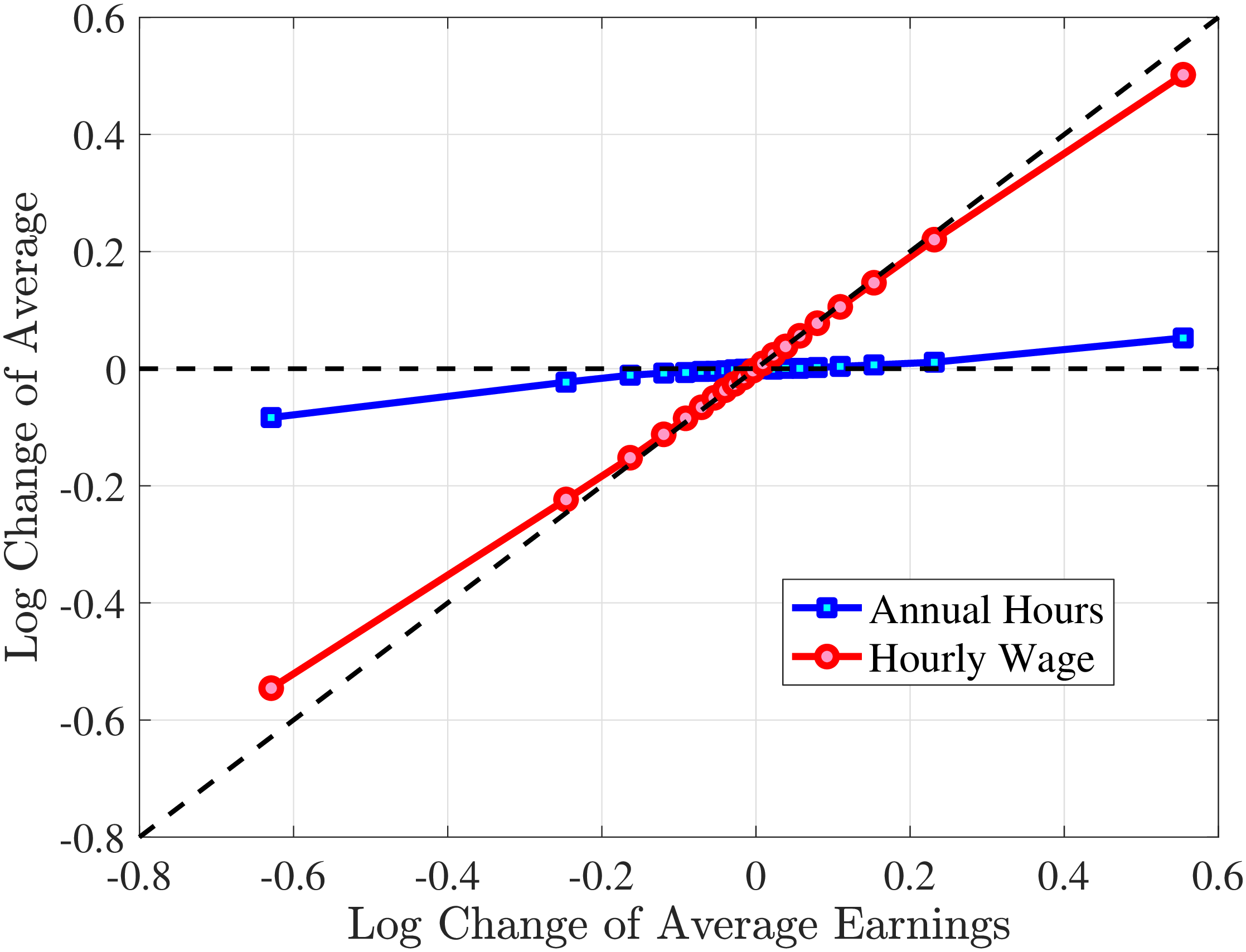
1st RE Decile

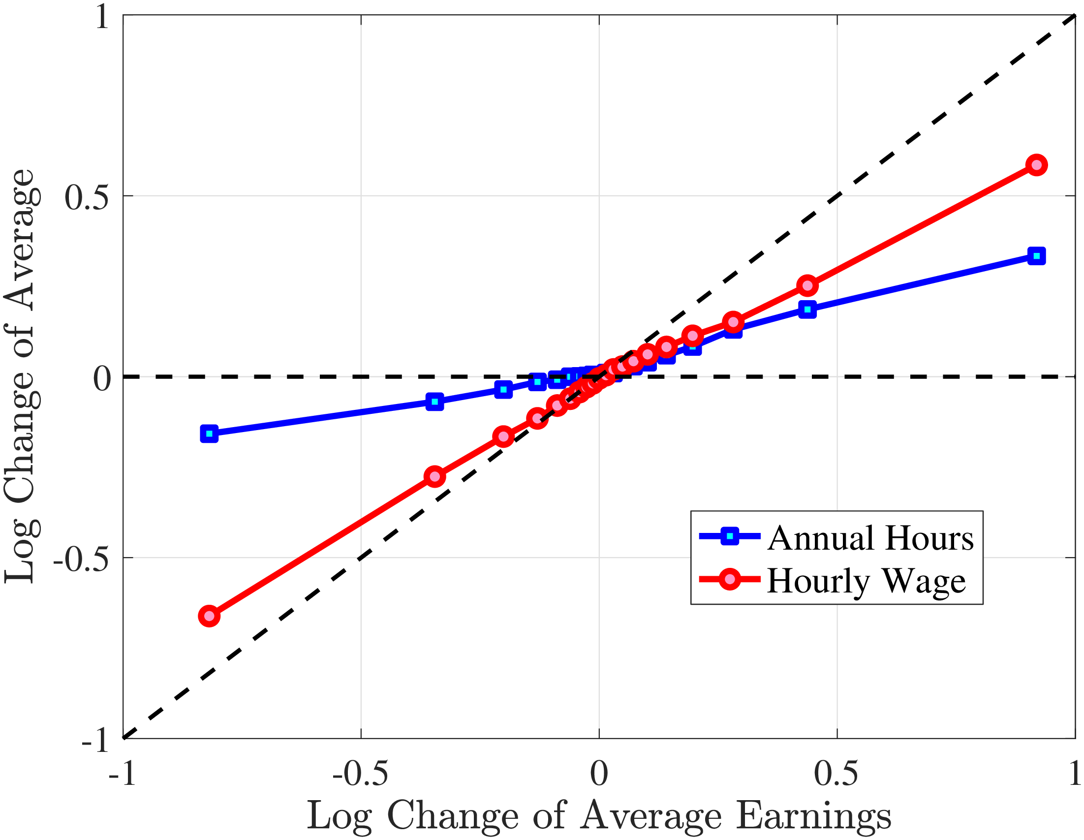
10th RE Decile

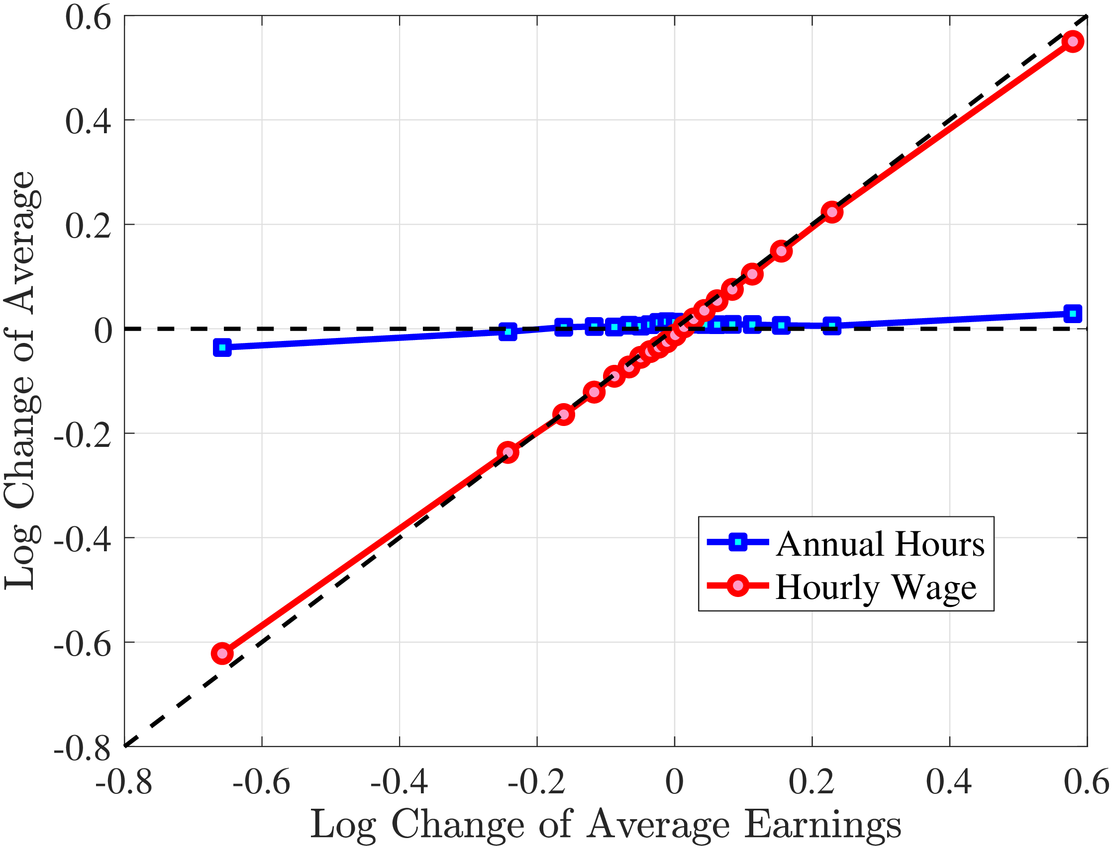
Figure D.11

–

Contribution of Hours and Hourly Wages to Male Earnings Shocks (Register Hours Data)

Note: The figure displays the one-year Representative-Agent change (i.e., log change of averages) for imputed hours and imputed wage rates for 20 different groups of prime-age males (ages 36–55) in the 1st RE decile (left panel) and 10th RE decile (right panel), plotted against their contemporaneous one-year log change in average annual earnings.

Figure: Figure D.11 – Contribution of Hours and Hourly Wages to Male Earnings Shocks (Register Hours Data)

10.2 Wage and Hours Growth Using Register Data on Hours

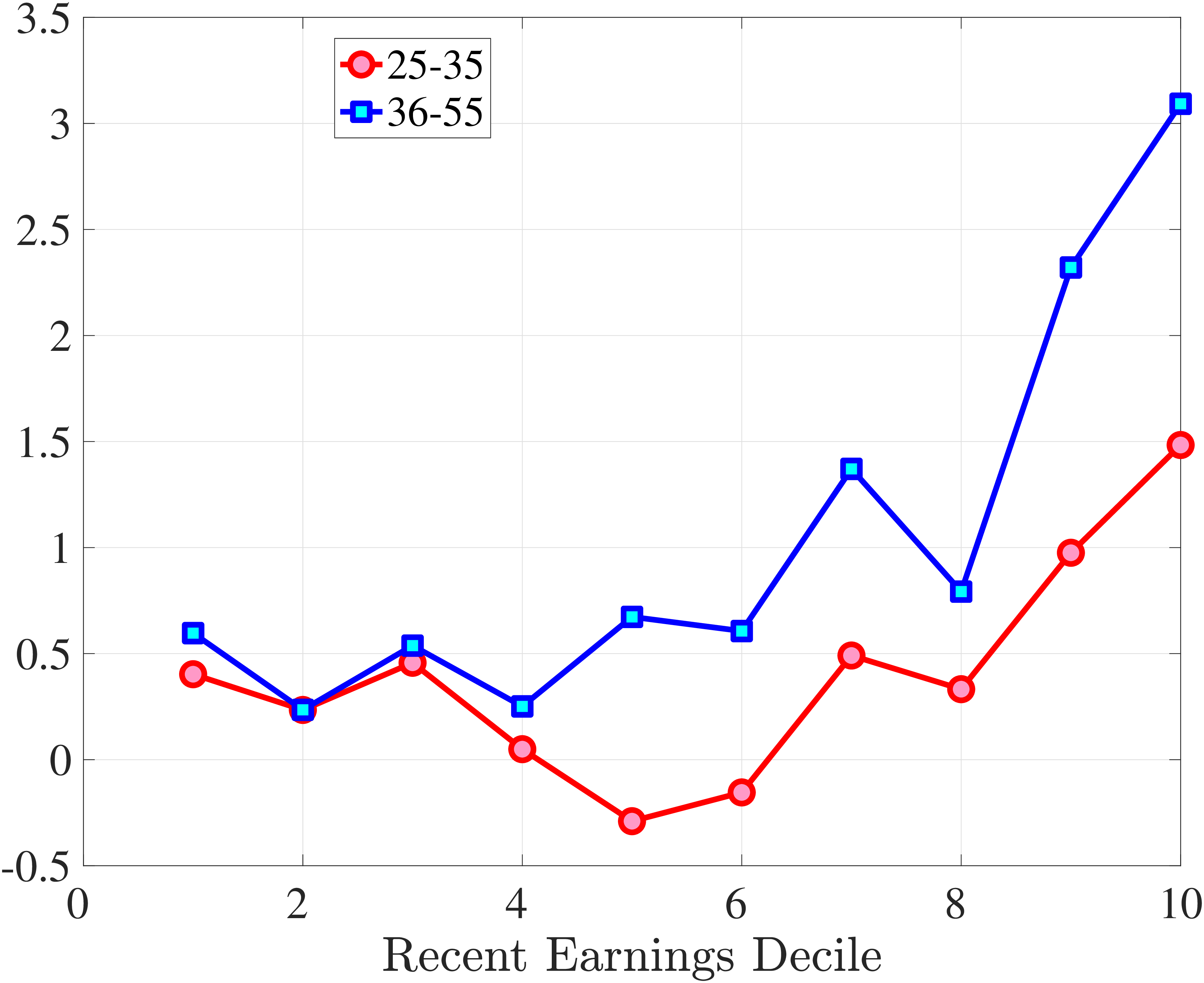(a) One-Year Hours Growth 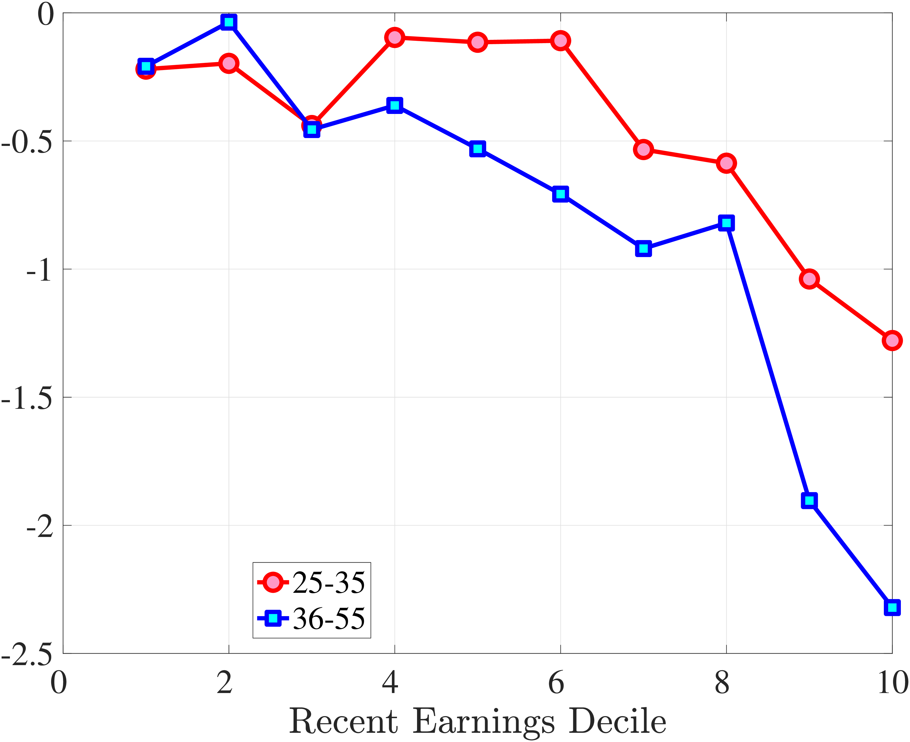(b) One-Year Hourly Wage Rate Growth

Figure D.12

–

Skewness of One-Year Male Hours and Hourly Wage Growth (Register Hours Data)

Note: The figure displays skewness for one-year hours growth (left panel) and one-year hourly wage rate growth (right panel) for two age groups.

Figure: Figure D.12 – Skewness of One-Year Male Hours and Hourly Wage Growth (Register Hours Data)

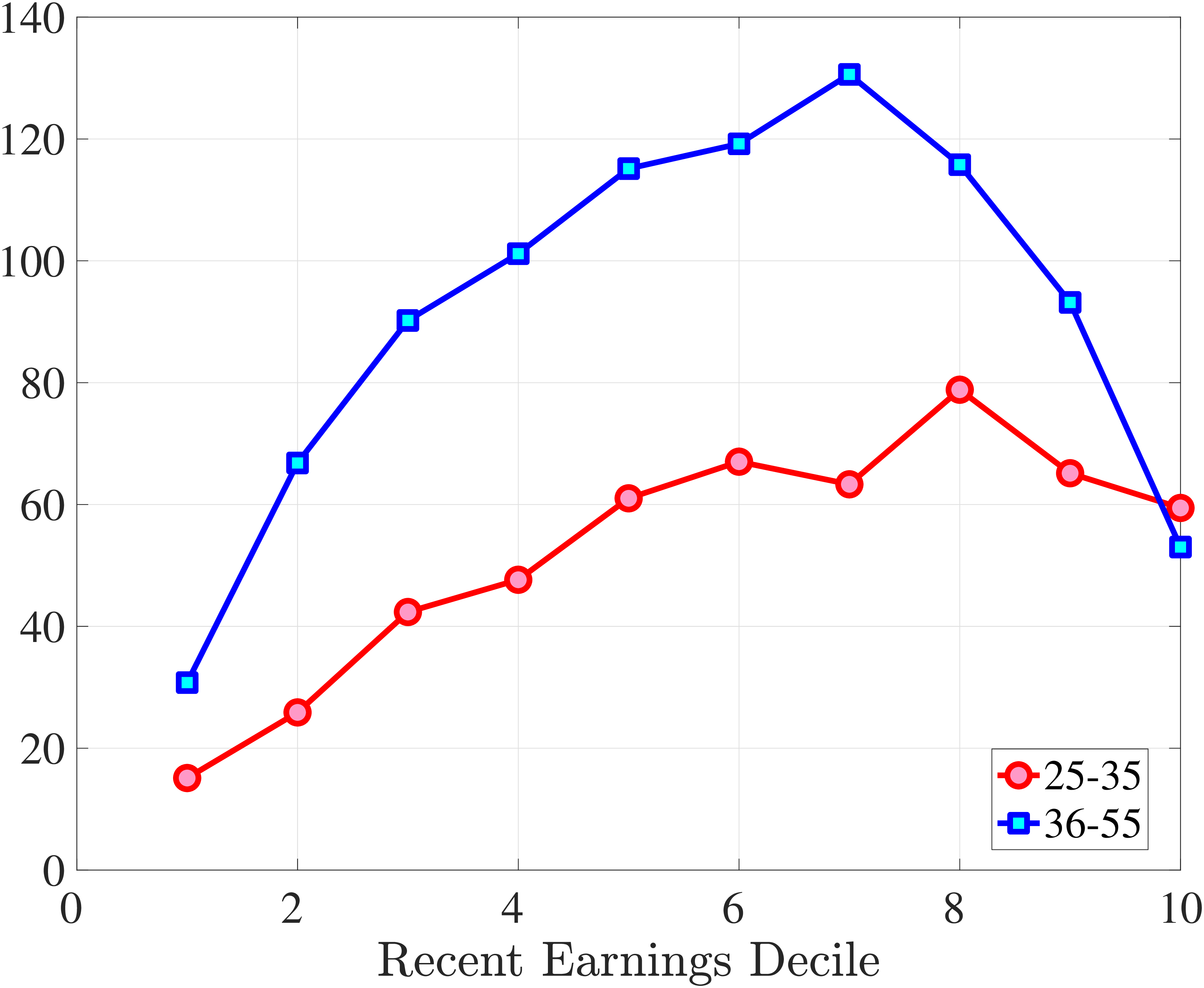(a) One-Year Hours Growth 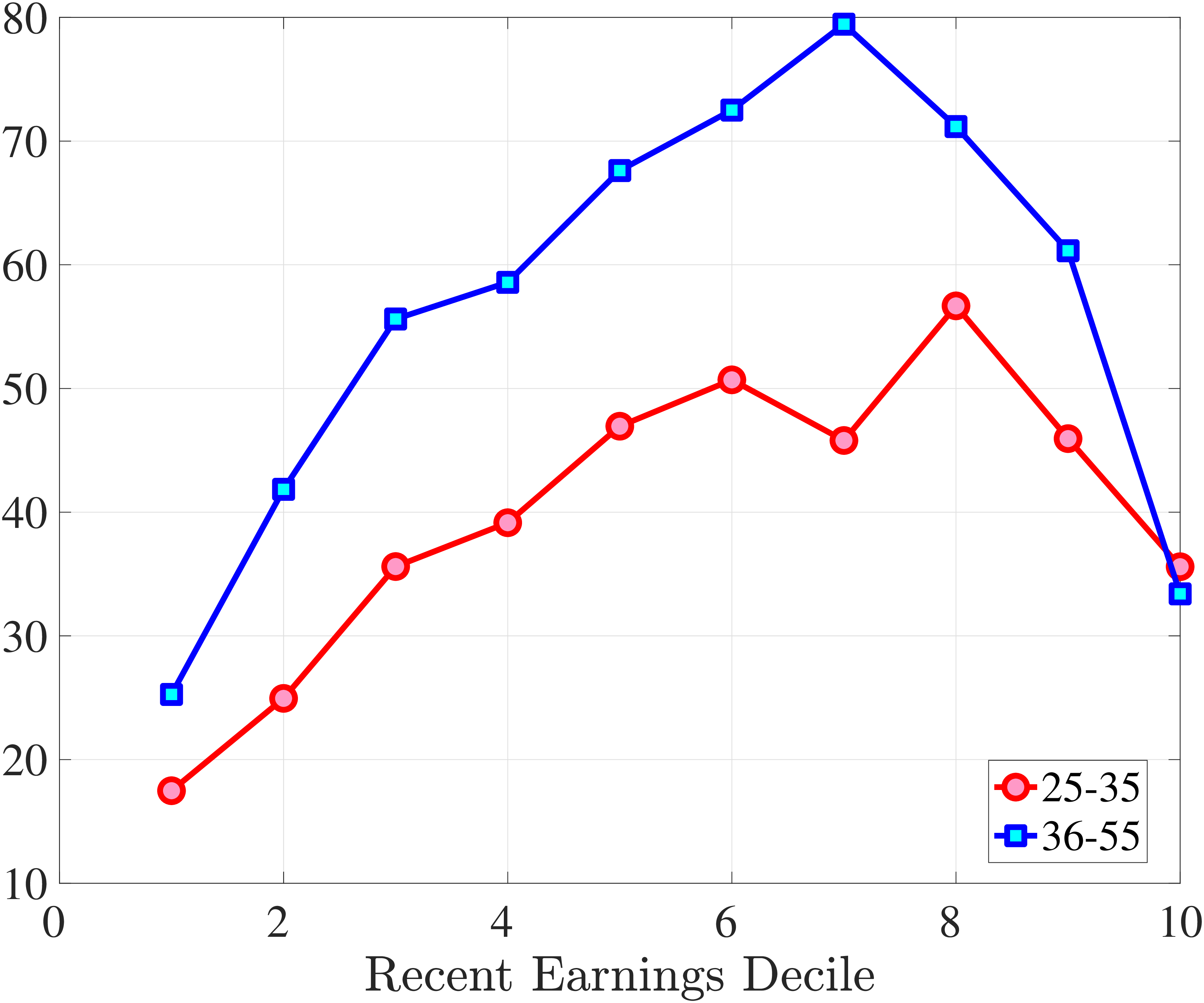(b) One-Year Wage Growth

Figure D.13

–

Kurtosis of One-Year Male Hours and Wage Rate Growth (Register Hours Data)

Note: The figure displays kurtosis for one-year hours growth (left panel) and one-year wage growth (right panel) for two age groups.

Figure: Figure D.13 – Kurtosis of One-Year Male Hours and Wage Rate Growth (Register Hours Data)

(a) Five-Year Hours Growth 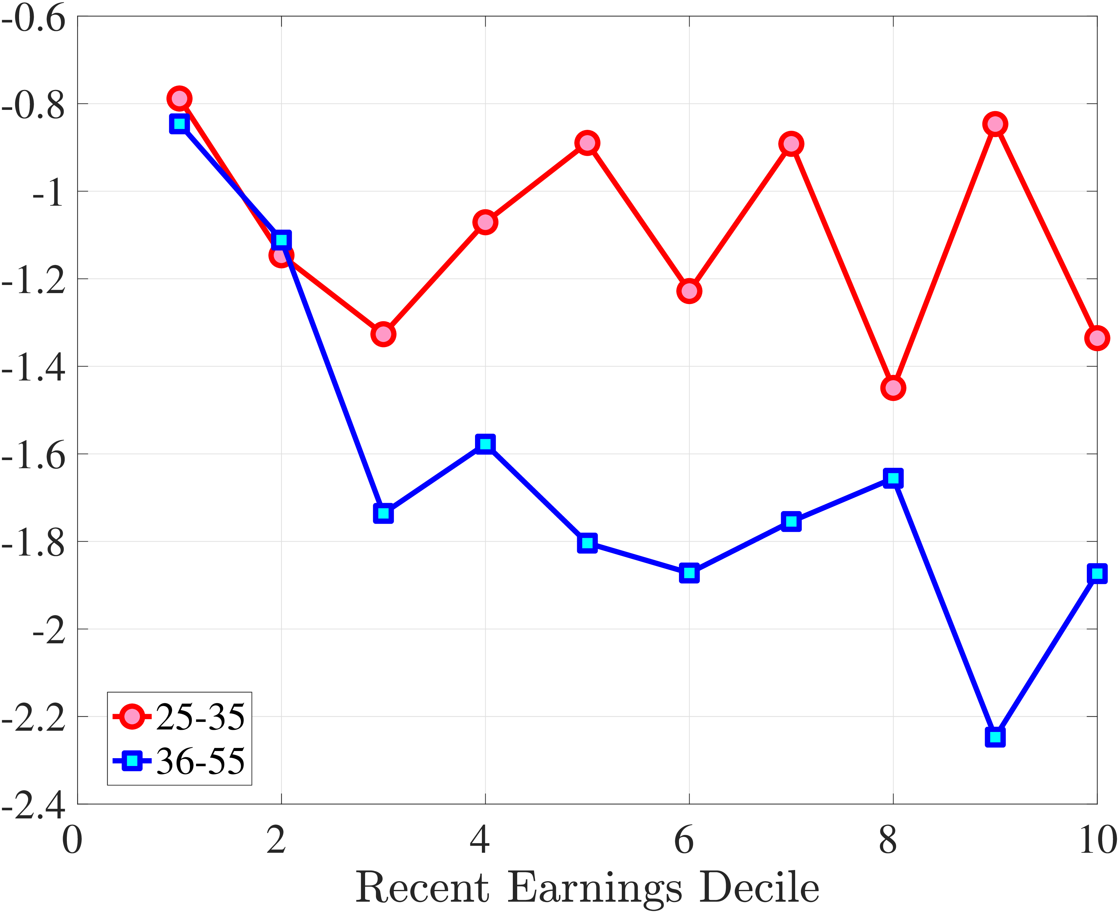(b) Five-Year Wage Growth

Figure D.14

–

Skewness of Five-Year Male Hours- and Wage- Growth (Register Hours)

Note: The figure displays skewness for five-year hours growth (left panel) and five-year hourly wage rate growth (right panel) for two age groups.

Figure: Figure D.14 – Skewness of Five-Year Male Hours- and Wage- Growth (Register Hours)

(a) Five-Year Hours Growth 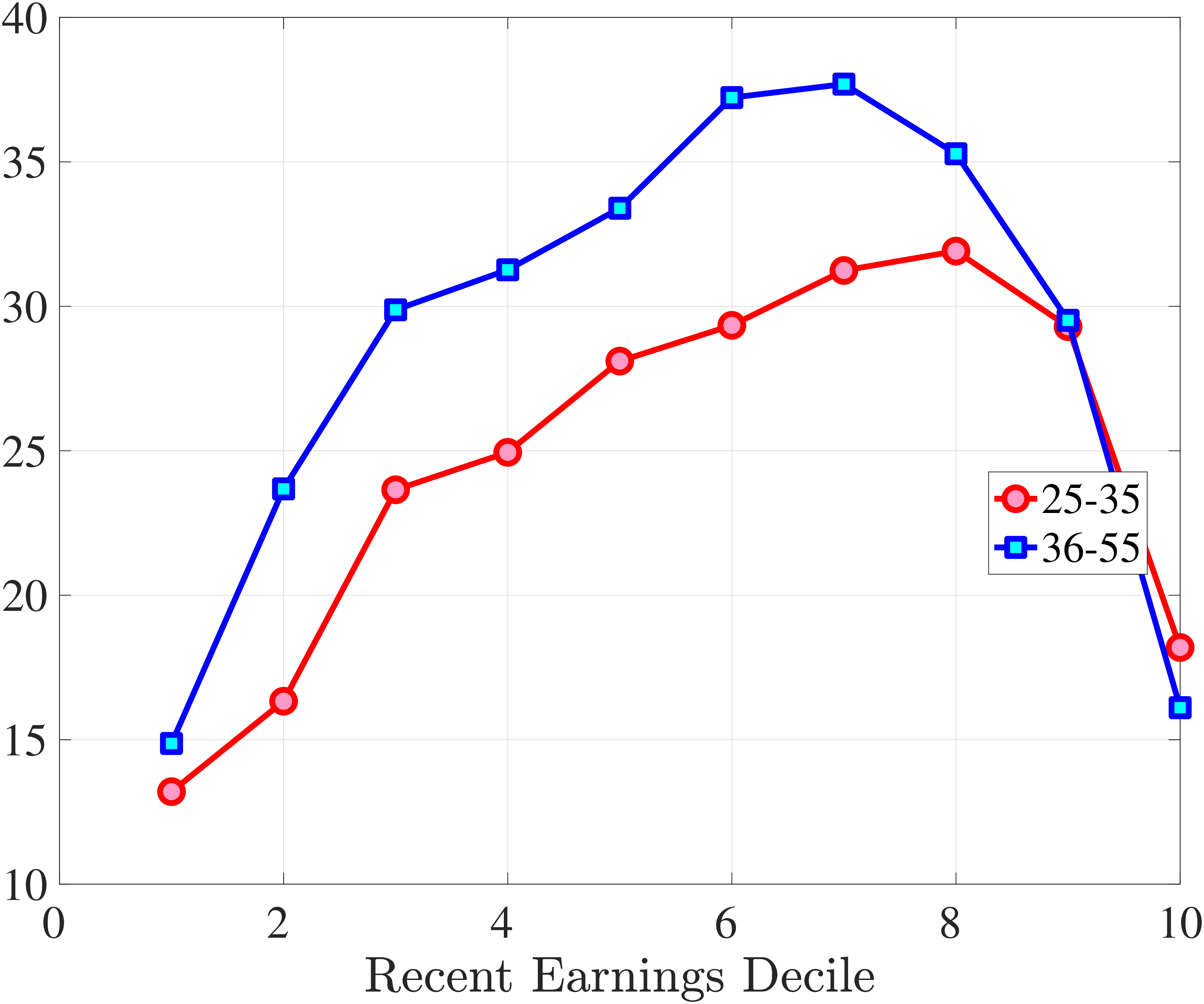(b) Five-Year Hourly Wage Rate Growth

Figure D.15

–

Kurtosis of Five-Year Male Hours and Wage Rate Growth (Register Hours)

Note: The figure displays kurtosis for five-year hours growth (left panel) and five-year hourly wage rate growth (right panel) for two age groups.

Figure: Figure D.15 – Kurtosis of Five-Year Male Hours and Wage Rate Growth (Register Hours)

10.3 Results Zooming in on Smaller Earnings Shocks

Figure D.16 – Contribution of Hours and Wage Rates to Earnings Shocks, 4th-7th RE Deciles (Smaller Earnings Shocks)

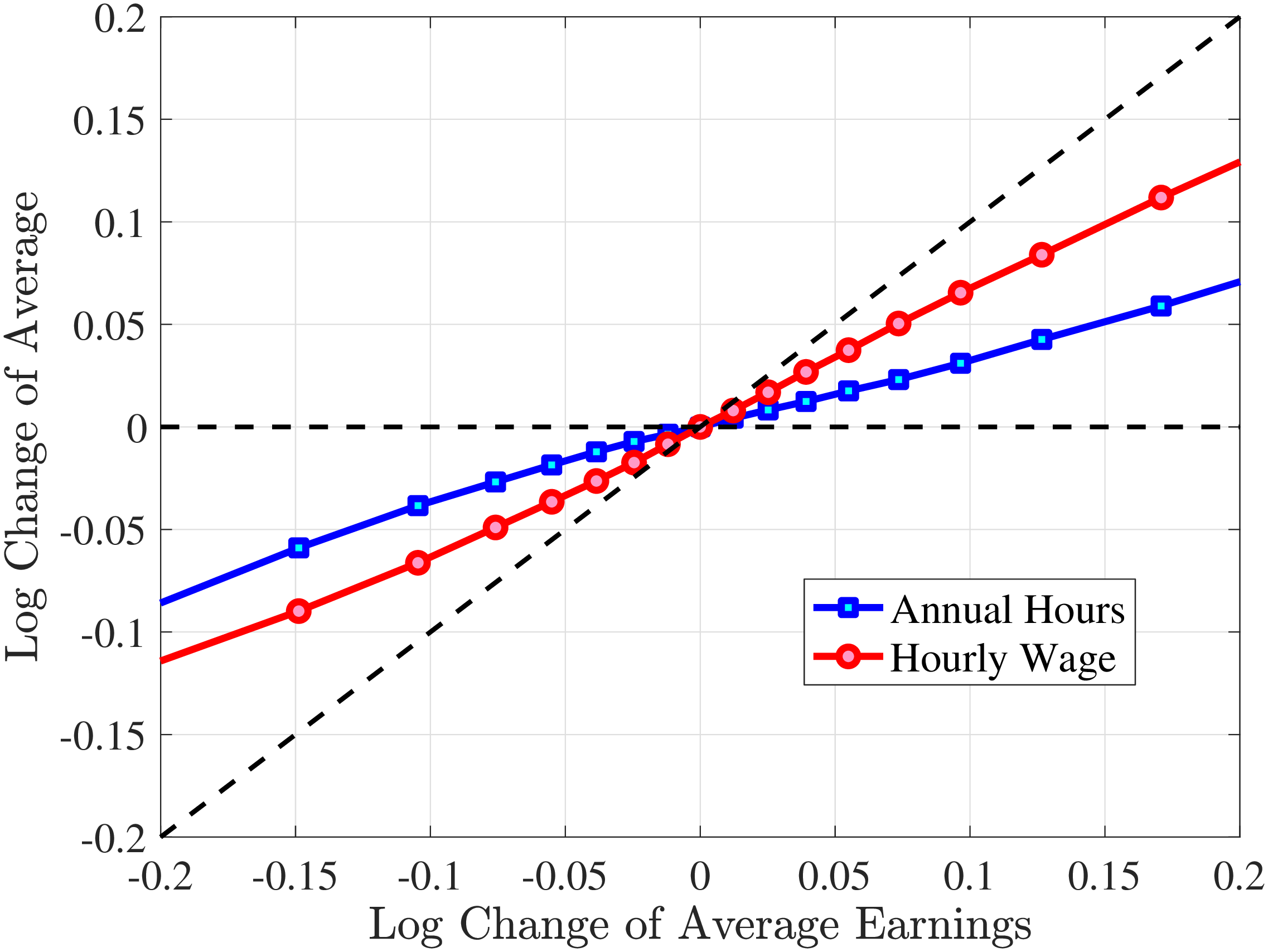
1st RE Decile

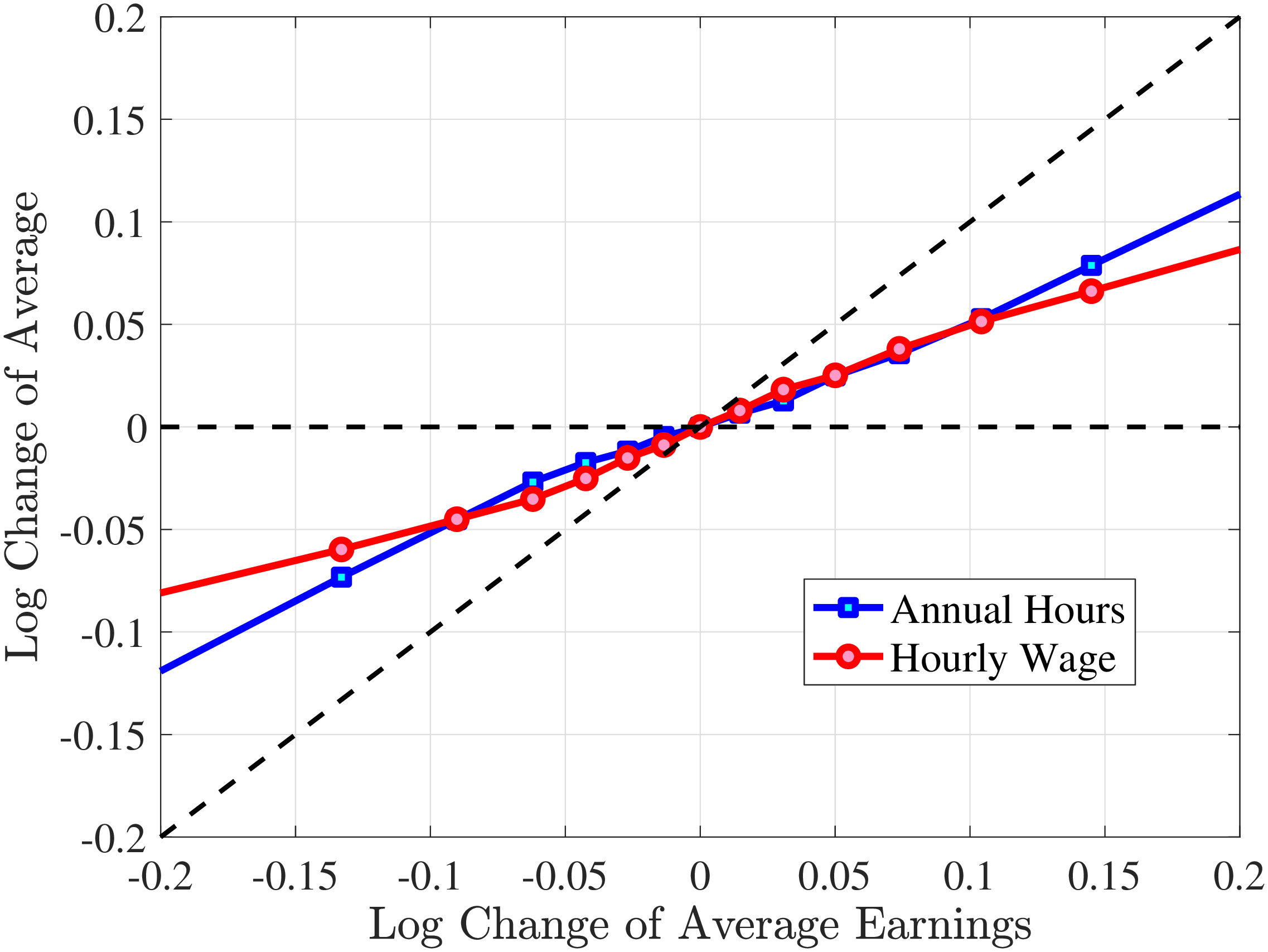
10th RE Decile

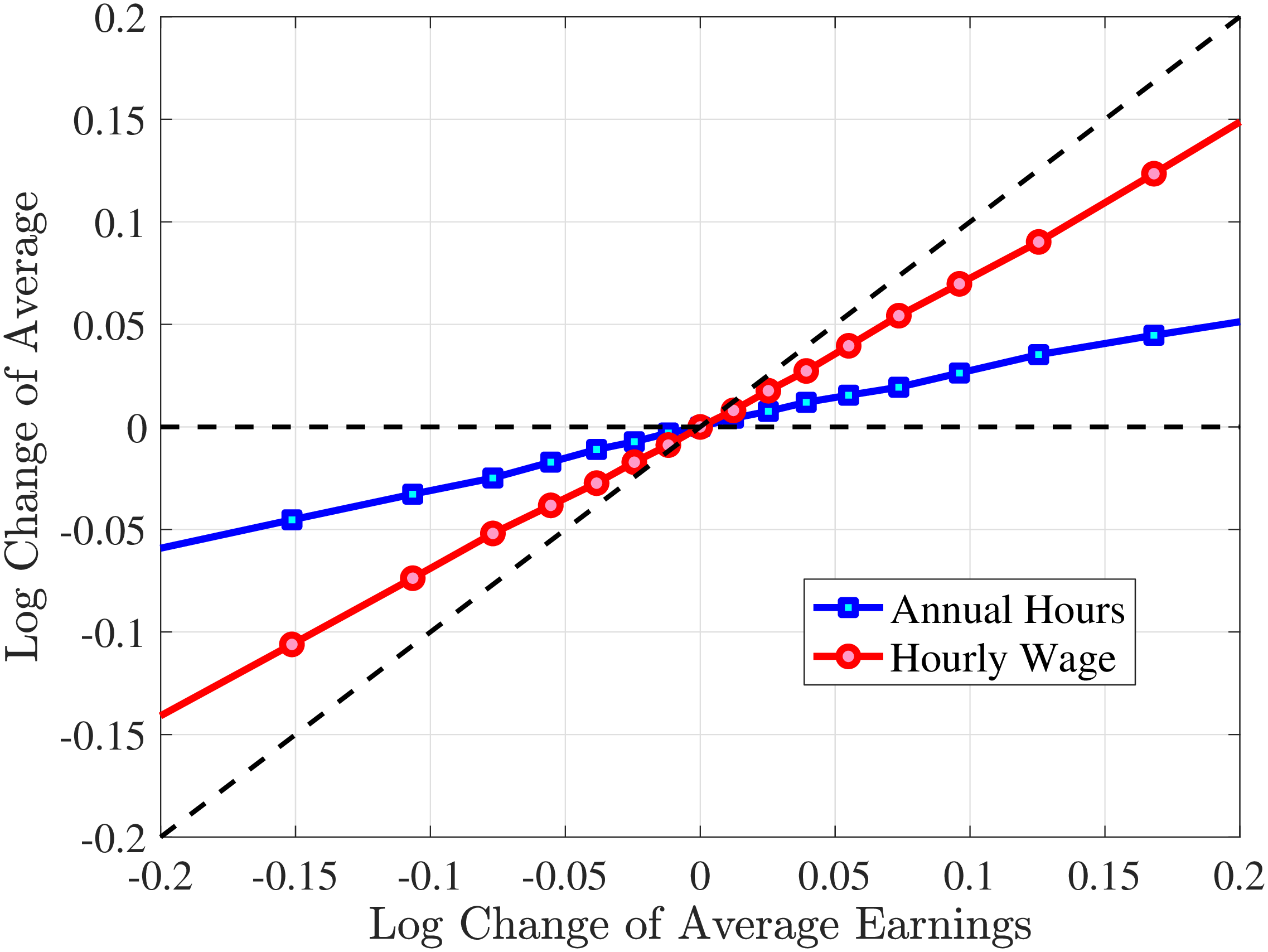
Figure D.17

–

Contribution of Hours and Wage Rates to Earnings Shocks (Smaller Earnings Shocks)

Note: The figure displays the one-year Representative-Agent change (log change of averages) for imputed hours and imputed wage rates for smaller earnings changes for prime-age males (ages 36–55) in the 1st RE decile (left panel) and 10th RE decile (right panel), plotted against their contemporaneous one-year log change in average annual earnings.

Figure: Figure D.17 – Contribution of Hours and Wage Rates to Earnings Shocks (Smaller Earnings Shocks)

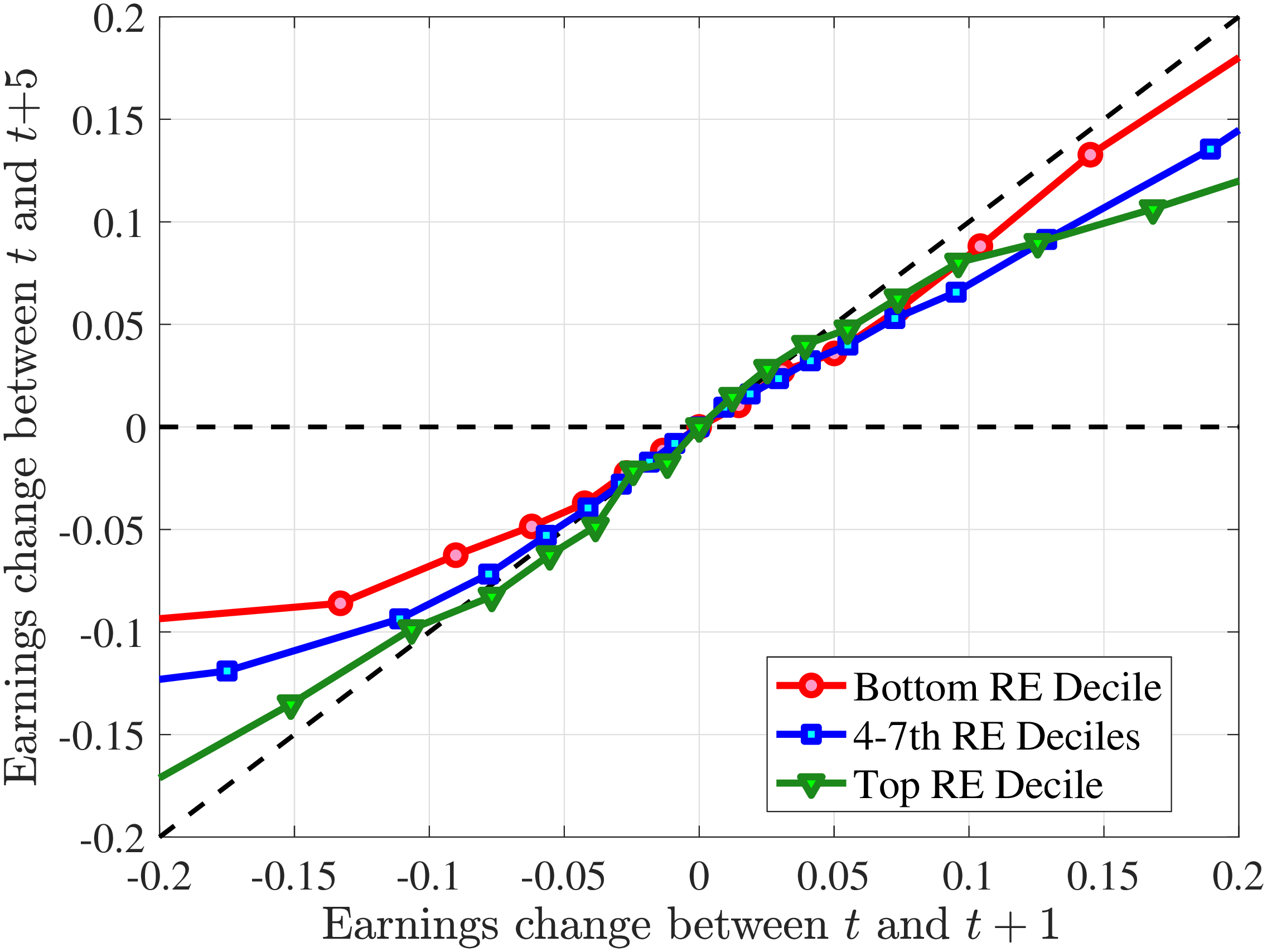
Figure D.18

–

Persistence of Earnings Changes, Prime Age Males (Smaller Earnings Shocks)

Note: The figure displays the five-year Representative-Agent change (i.e., log change of averages) in earnings of prime-age males (ages 36–55) in the 1st RE decile, 4th-7th RE deciles, and 10th RE decile, plotted against their respective one-year log change in average annual earnings.

Figure: Figure D.18 – Persistence of Earnings Changes, Prime Age Males (Smaller Earnings Shocks)

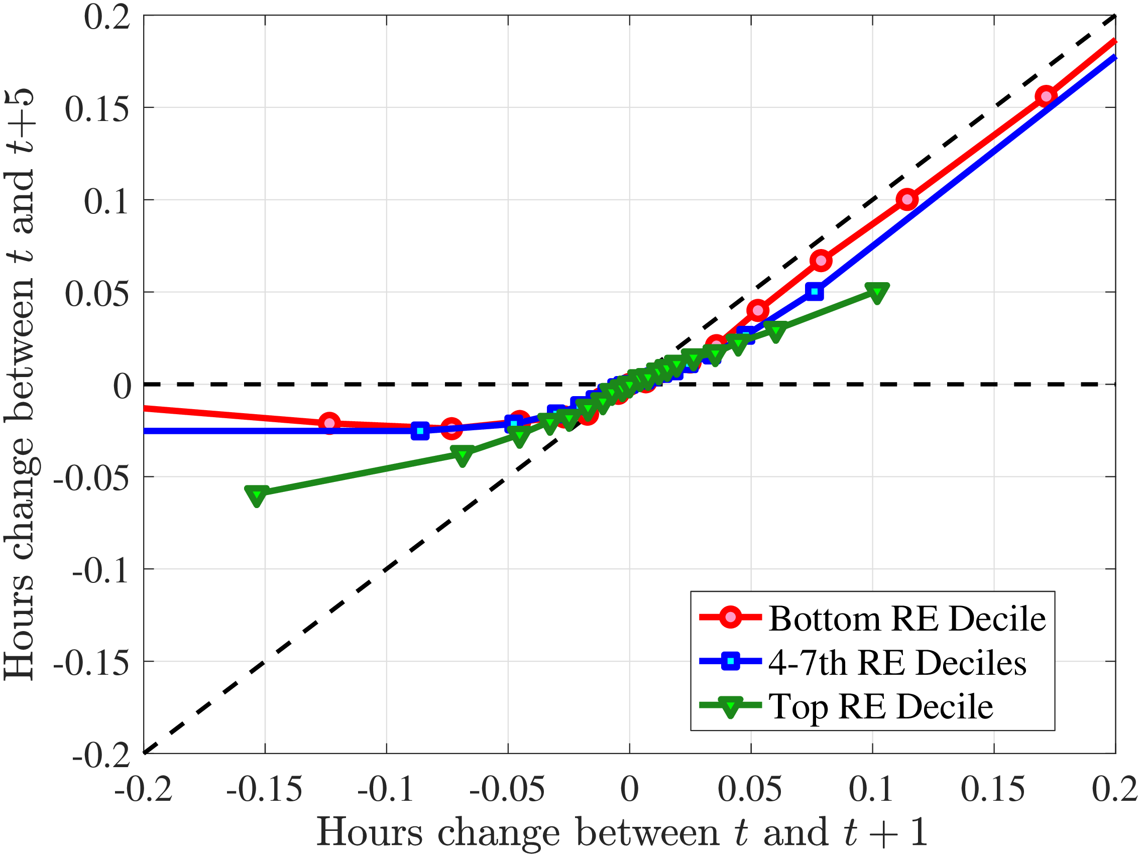(a) Annual Hours 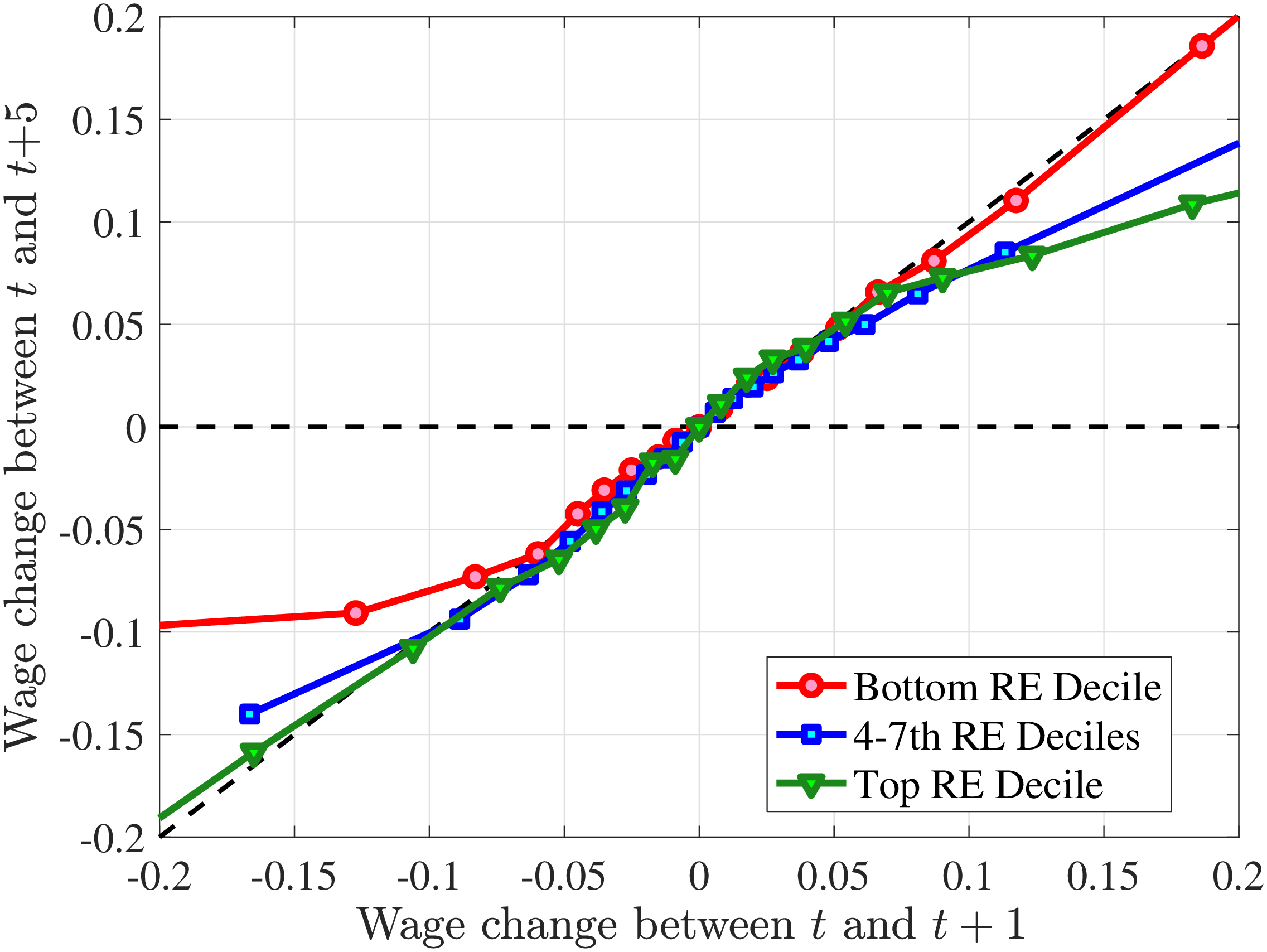(b) Hourly Wage

Figure D.19

–

Persistence of Hours and Wage Changes (Smaller Earnings Shocks)

Note: The left panel displays the five-year Representative-Agent change (i.e., log change of averages) in imputed annual hours and wages of prime-age males (ages 36–55) in the 1st RE decile (red line), 4th-7th RE deciles (blue line), and 10th RE decile (green line), plotted against their respective one-year log change in imputed annual average hours. The right panel displays the corresponding figure for imputed hourly wage rates.

Figure: Figure D.19 – Persistence of Hours and Wage Changes (Smaller Earnings Shocks)

11 Results for Females

11.1 Higher-Order Moments of Earnings Growth

Figure E.1 displays the variance of earnings growth for women. The results for women above 35 are both qualitatively and quantitatively quite similar to those for men. One difference is that the U-shape with higher variance for the highest earners is less pronounced for women. Women between ages 25 and 35 have more volatile earnings shocks than males across all RE groups and there is no decline in volatility by RE. In Table E.1, we show that parental leave is a key driver of large female earnings shocks, and this is likely to explain the high volatility of earnings growth for young women.

Figure E.2 displays the skewness of earnings growth for females. The negative skewness is less pronounced for younger women than it is for men and varies less by earnings group. For older women (ages 46–55), the negative skewness is similar to that of men in the same age group. However, we do not observe the U-shape for high top earners.

In Figure E.4, we plot the kurtosis of one-year earnings growth (left) and five-year earnings growth (right) for women. For young women, the kurtosis of earnings growth is generally much lower than for young men, and the increase by earnings group is less pronounced. For the younger group, ages 25–35, the kurtosis of one-year earnings growth is close to 3 (the value for a normal distribution). For older women (ages 45–55), the kurtosis of earnings growth is high and sharply increasing in recent earnings, with an inverted U-shape for top earners.

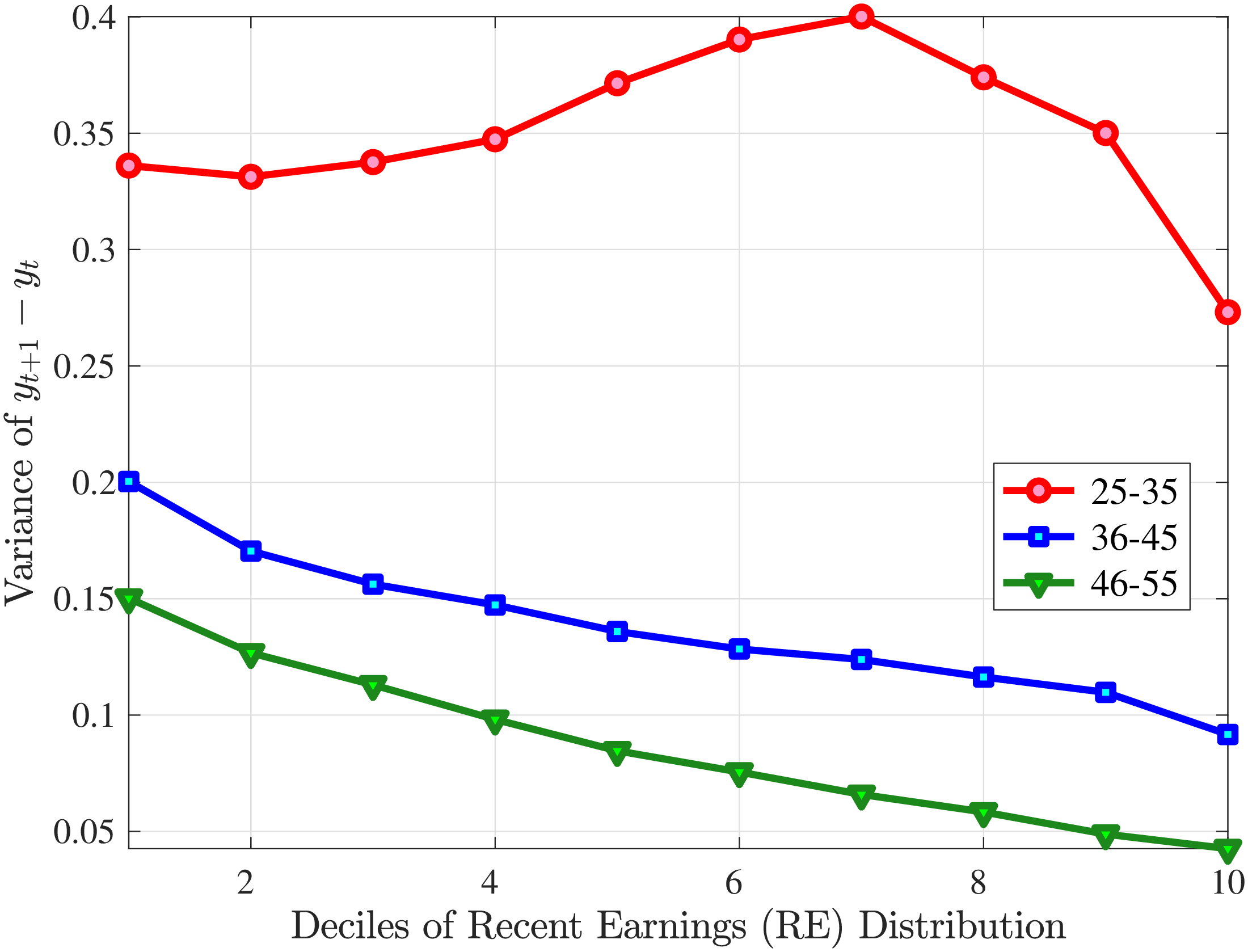
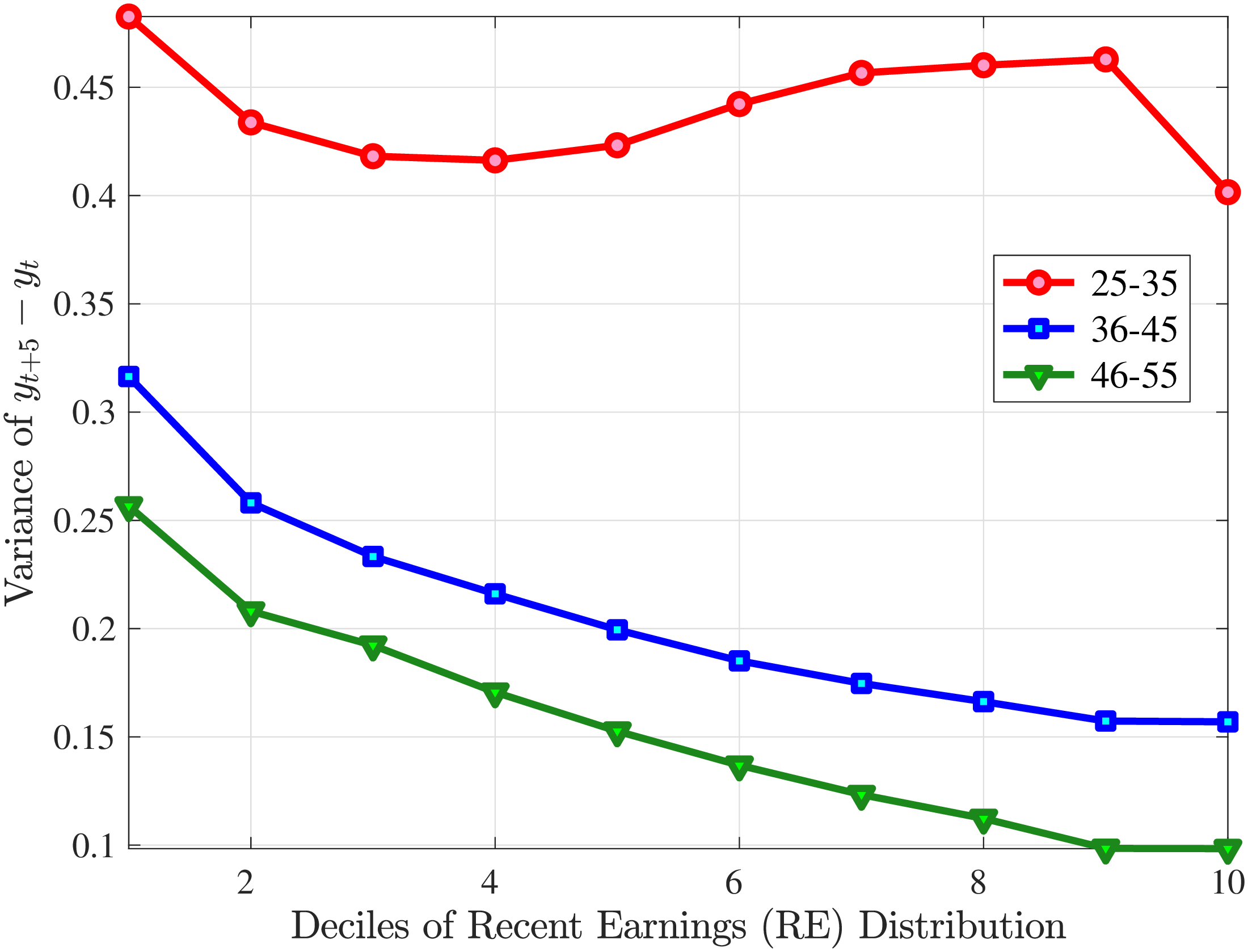
Figure E.1

–

Variance of Female Earnings Growth

Note:

The figure displays the variance of one-year (left) and five-year (right) earnings growth for females by age and RE

decile.

Figure: Figure E.1 – Variance of Female Earnings Growth

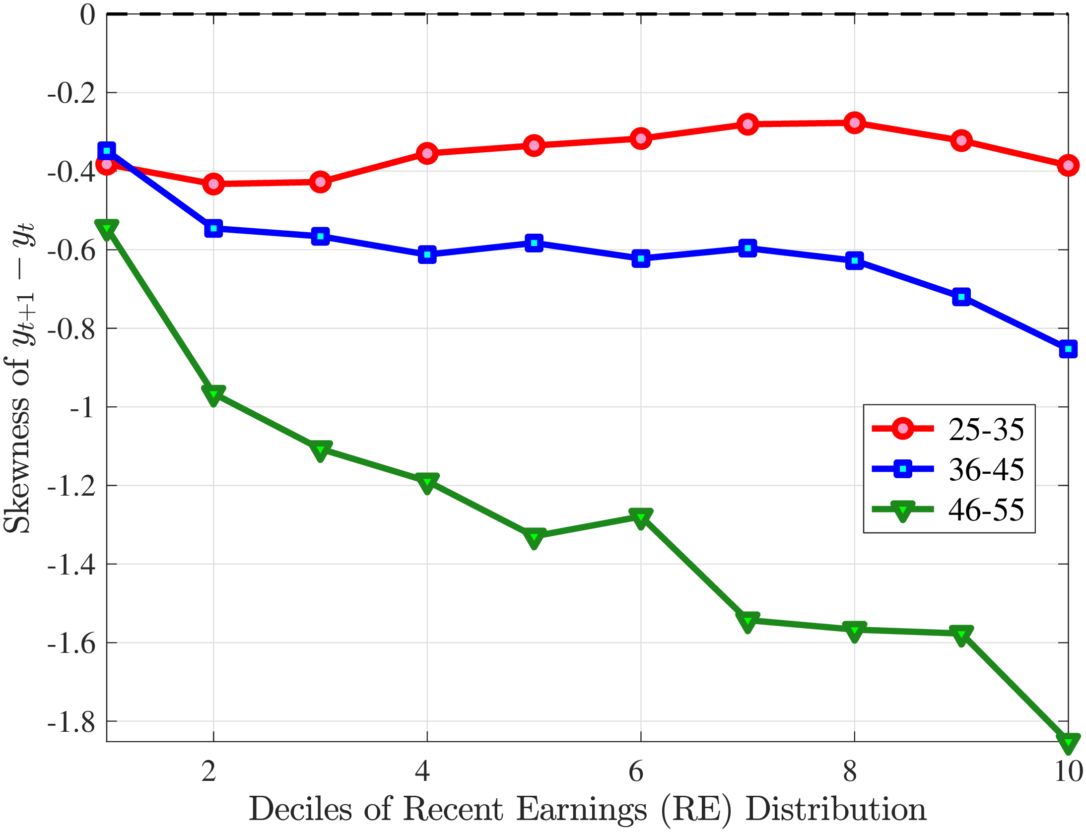
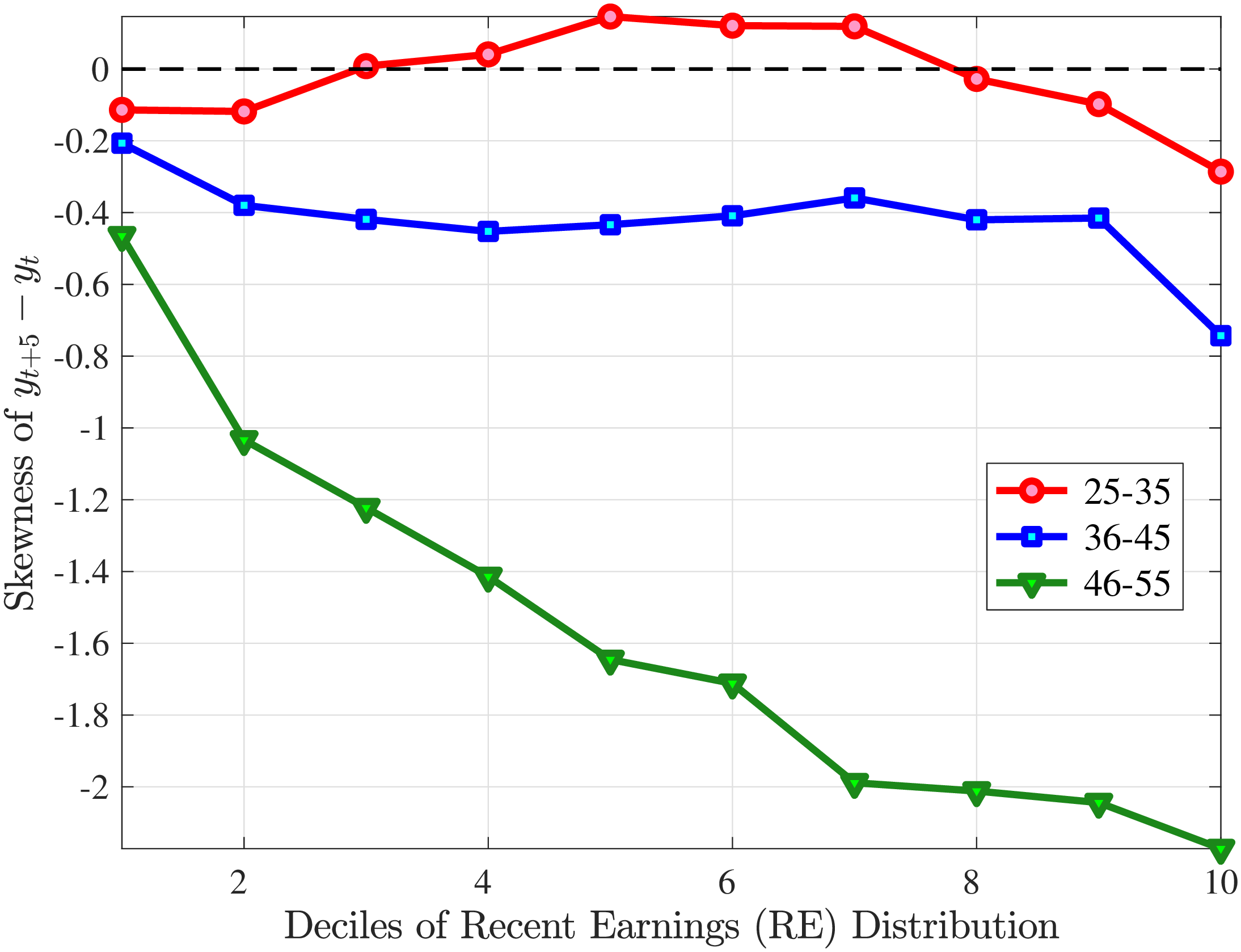
Figure E.2

–

Skewness of Female Earnings Growth

Note:

The figure displays the skewness of one-year (left) and five-year (right) earnings growth for females by age and

RE.

Figure: Figure E.2 – Skewness of Female Earnings Growth

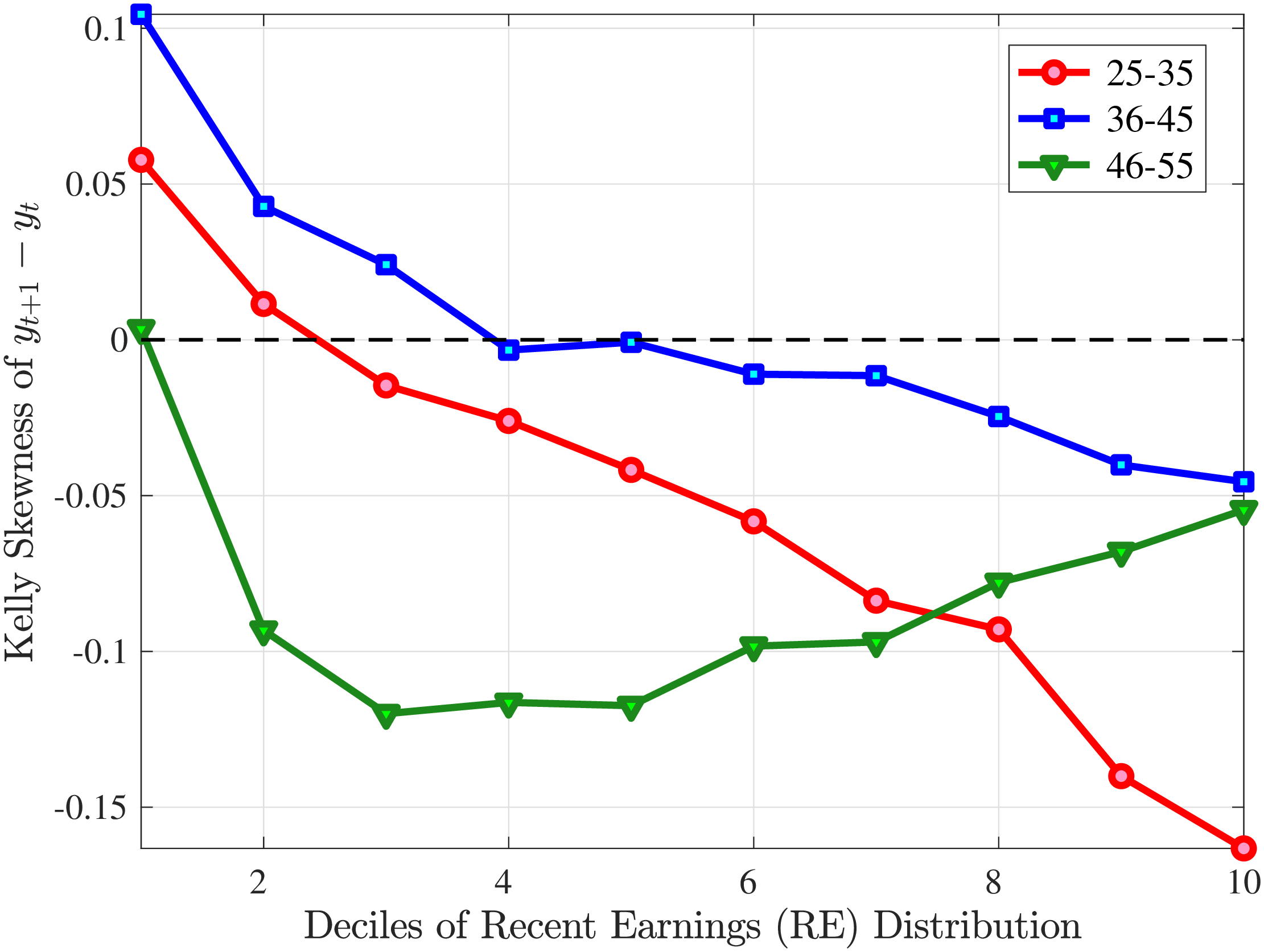
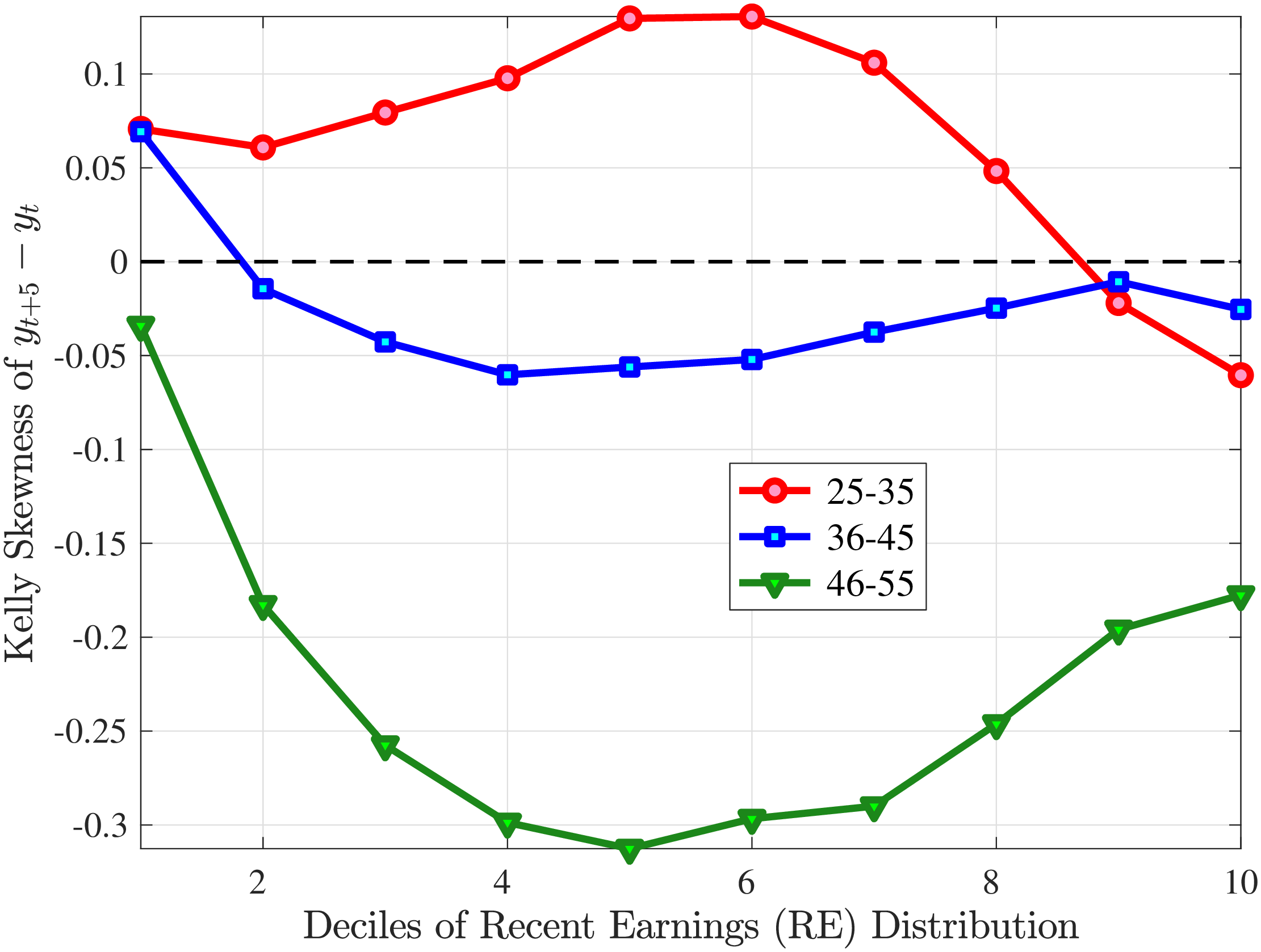
Figure E.3

–

Kelly Skewness of Female Earnings Growth

Note:

The figure displays the Kelly skewness of one-year (left) and five-year (right) earnings growth for females by age and

RE.

Figure: Figure E.3 – Kelly Skewness of Female Earnings Growth

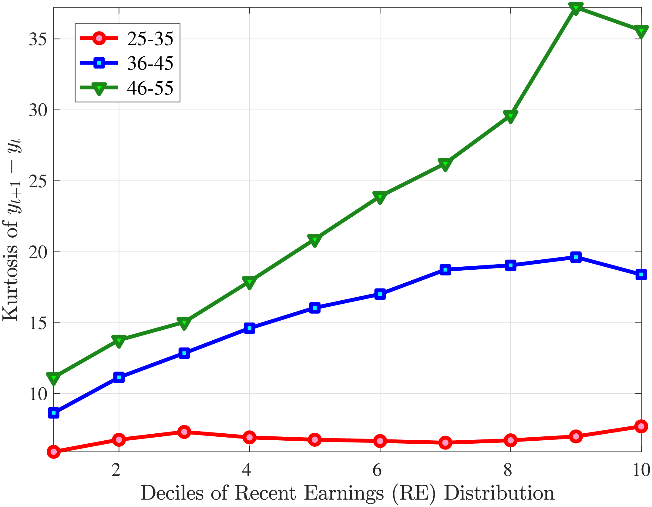
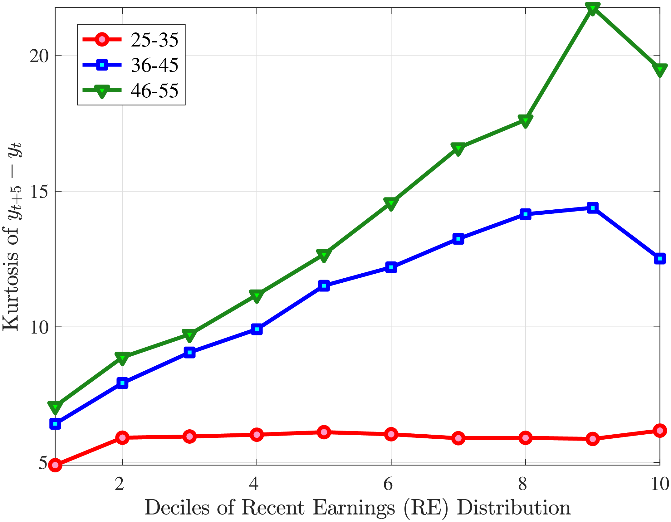
Figure E.4

–

Kurtosis of Female Earnings Growth

Note:

The figure displays the kurtosis of one-year (left) and five-year (right) earnings growth for females by age and

RE.

Figure: Figure E.4 – Kurtosis of Female Earnings Growth

11.2 Life Events Associated with Large Female Earnings Shocks

Table E.1 displays the fraction of female workers with large and small, positive and negative earnings changes that experience certain events. A key difference between women and men is that one of the most frequent events experienced by women with large earnings changes is parental leave, which is associated with 29% of negative changes and 28% of positive changes. Moreover, long-term sickness is associated with 27% of negative changes and 26% of positive changes, and change of employer is associated with 13% of negative changes and 20% of positive changes. Another key difference between men and women is that men with large earnings shocks tend to experience larger changes in hourly wage and smaller changes in hours worked. For example, the log hourly wage rate for women with large income shocks declines by just 0.18 for negative shocks and increases by just 0.21 for positive shocks. The average change in log hours, however, is -0.78 and 0.71 for women with large negative and positive shocks, respectively. For men with large earnings shocks, the average change in log wage rates is -0.44 and 0.45 and the average change in log hours is -0.40 and 0.40 for positive and negative earnings shocks, respectively.

					Annual Earnings Change, $\Delta y\in$
All		One-Year Earnings Loss			One-Year Earnings Gain
Life-cycle event		$\lt -0.5$	$[-0.5,-0.25)$	$[-0.25,0.0)$	$[0.0,0.25)$	$[0.25,0.5)$	$\geq 0.5$
into/out of		(1)	(2)	(3)	(4)	(5)	(6)
(1)	Unemployment	0.04	0.04	0.01	0.02	0.05	0.04
(2)	Long-term sick	0.27	0.27	0.12	0.12	0.24	0.26
(3)	Part-time	0.09	0.09	0.05	0.08	0.14	0.15
(4)	Parental leave	0.29	0.18	0.00	0.01	0.20	0.28
(5)	Firm change	0.13	0.15	0.10	0.11	0.19	0.20
(6)	$\mathbb{E}\left [\Delta _{\log}^{1}h_{t}^{i}\right]$	-0.78	-0.55	-0.04	0.05	0.50	0.71
(7)	$\mathbb{E}\left [\Delta _{\log}^{5}h_{t}^{i}\right]$	-0.13	-0.12	-0.07	-0.02	0.46	0.68
(8)	$\mathbb{E}\left [\Delta _{\log}^{1}w_{t}^{i}\right]$	-0.18	-0.14	-0.03	0.03	0.14	0.21
(9)	$\mathbb{E}\left [\Delta _{\log}^{5}w_{t}^{i}\right]$	-0.08	-0.08	-0.04	0.02	0.11	0.18
(10)	# of Obs.	357,736	671,342	2,529,768	2,133,763	732,965	384,150
Lowest decile (RE=1)		(1)	(2)	(3)	(4)	(5)	(6)
(1)	Unemployment	0.07	0.07	0.03	0.03	0.06	0.06
(2)	Long-term sick	0.25	0.24	0.14	0.11	0.15	0.14
(3)	Part-time	0.12	0.10	0.05	0.09	0.18	0.25
(4)	Parental leave	0.12	0.04	0.00	0.01	0.03	0.08
(5)	Firm change	0.23	0.22	0.15	0.17	0.27	0.35
(6)	$\mathbb{E}\left [\Delta _{\log}^{1}h_{t}^{i}\right]$	-0.51	-0.21	-0.05	0.05	0.22	0.48
(7)	$\mathbb{E}\left [\Delta _{\log}^{5}h_{t}^{i}\right]$	-0.02	0.01	0.02	0.09	0.25	0.50
(8)	$\mathbb{E}\left [\Delta _{\log}^{1}w_{t}^{i}\right]$	-0.37	-0.14	-0.03	0.04	0.13	0.35
(9)	$\mathbb{E}\left [\Delta _{\log}^{5}w_{t}^{i}\right]$	-0.04	-0.04	-0.02	0.03	0.12	0.35
(10)	# of Obs.	17,033	21,290	119,260	151,221	44,480	37,994
Top decile (RE=10)		(1)	(2)	(3)	(4)	(5)	(6)
(1)	Unemployment	0.03	0.03	0.00	0.01	0.02	0.02
(2)	Long-term sick	0.24	0.23	0.10	0.12	0.23	0.27
(3)	Part-time	0.09	0.10	0.05	0.06	0.10	0.10
(4)	Parental leave	0.35	0.13	0.01	0.02	0.18	0.36
(5)	Firm change	0.19	0.22	0.13	0.13	0.22	0.21
(6)	$\mathbb{E}\left [\Delta _{\log}^{1}h_{t}^{i}\right]$	-0.97	-0.32	-0.03	0.03	0.32	0.88
(7)	$\mathbb{E}\left [\Delta _{\log}^{5}h_{t}^{i}\right]$	-0.17	-0.12	-0.11	-0.05	0.27	0.84
(8)	$\mathbb{E}\left [\Delta _{\log}^{1}w_{t}^{i}\right]$	0.09	-0.03	-0.04	0.04	0.03	-0.04
(9)	$\mathbb{E}\left [\Delta _{\log}^{5}w_{t}^{i}\right]$	-0.15	-0.15	-0.04	0.04	-0.06	-0.11
(10)	# of Obs.	29,724	30,992	299,107	250,623	25,216	19,040

Table E.1 – Important Life Cycle Events Associated with Earnings Changes (Females)

11.3 Job Stayers and Job Switchers

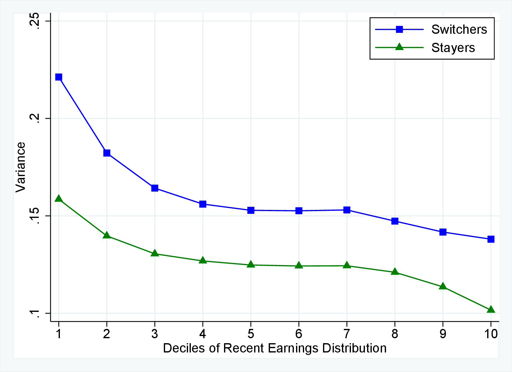
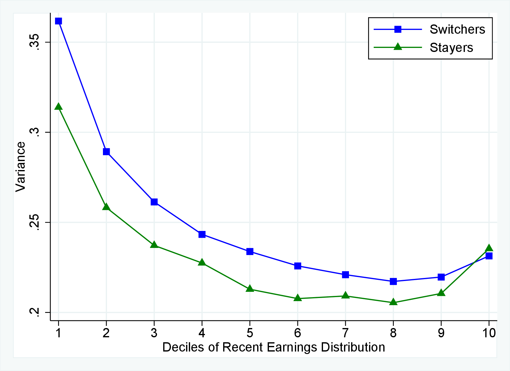
Figure: Figure E.5 – Variance of Female Earnings Growth, Ages 25-55

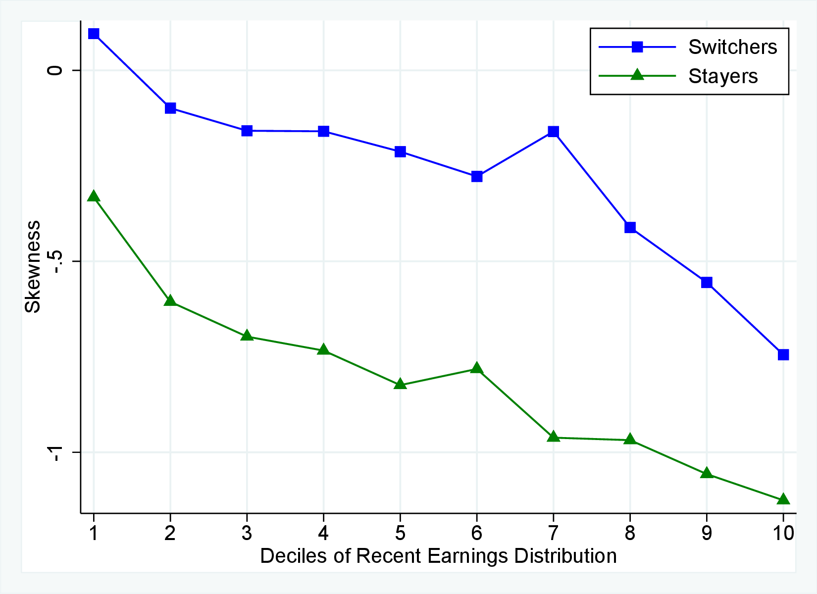
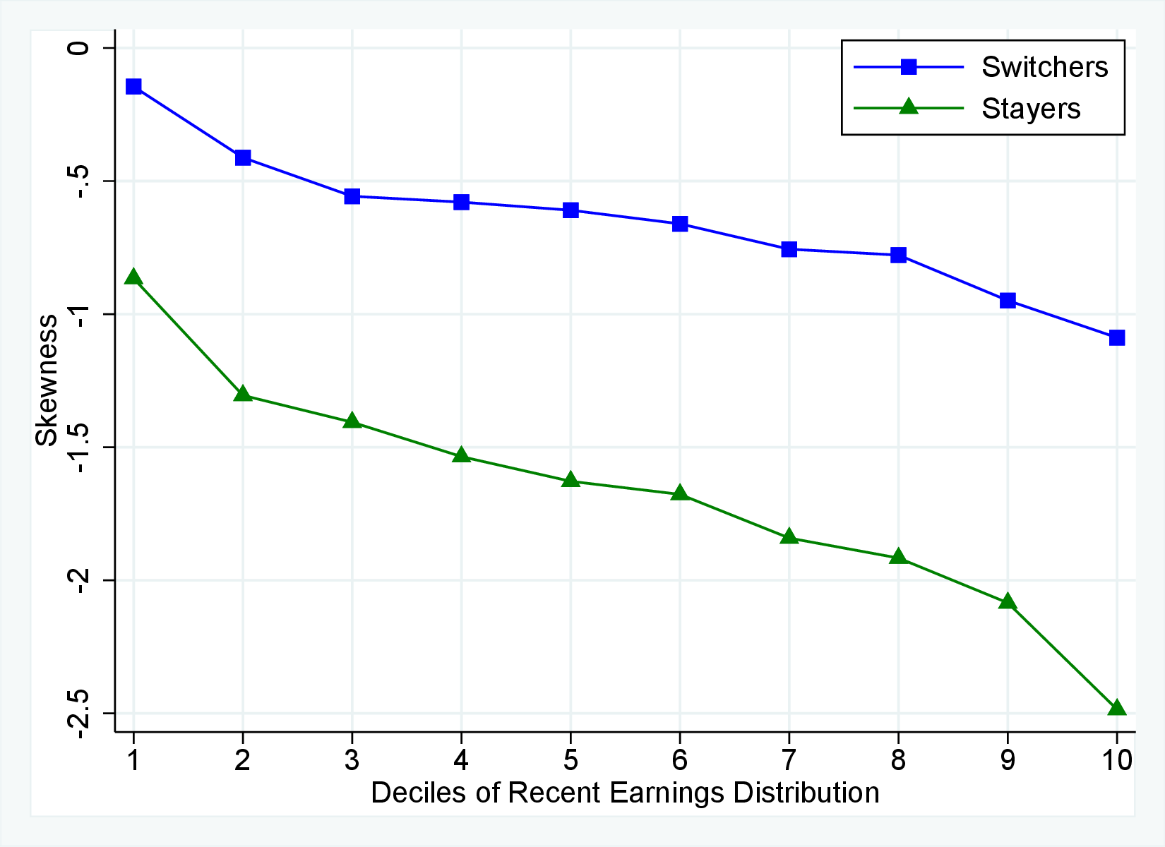
Figure: Figure E.6 – Skewness of Female Earnings Growth, Ages 25-55

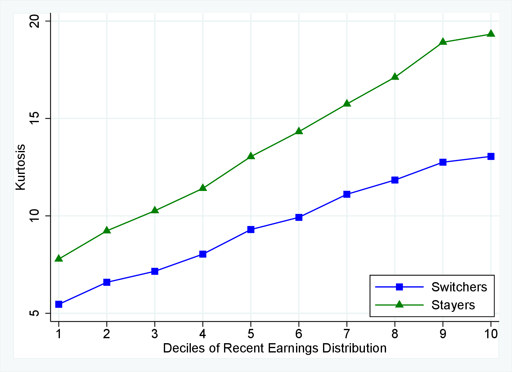
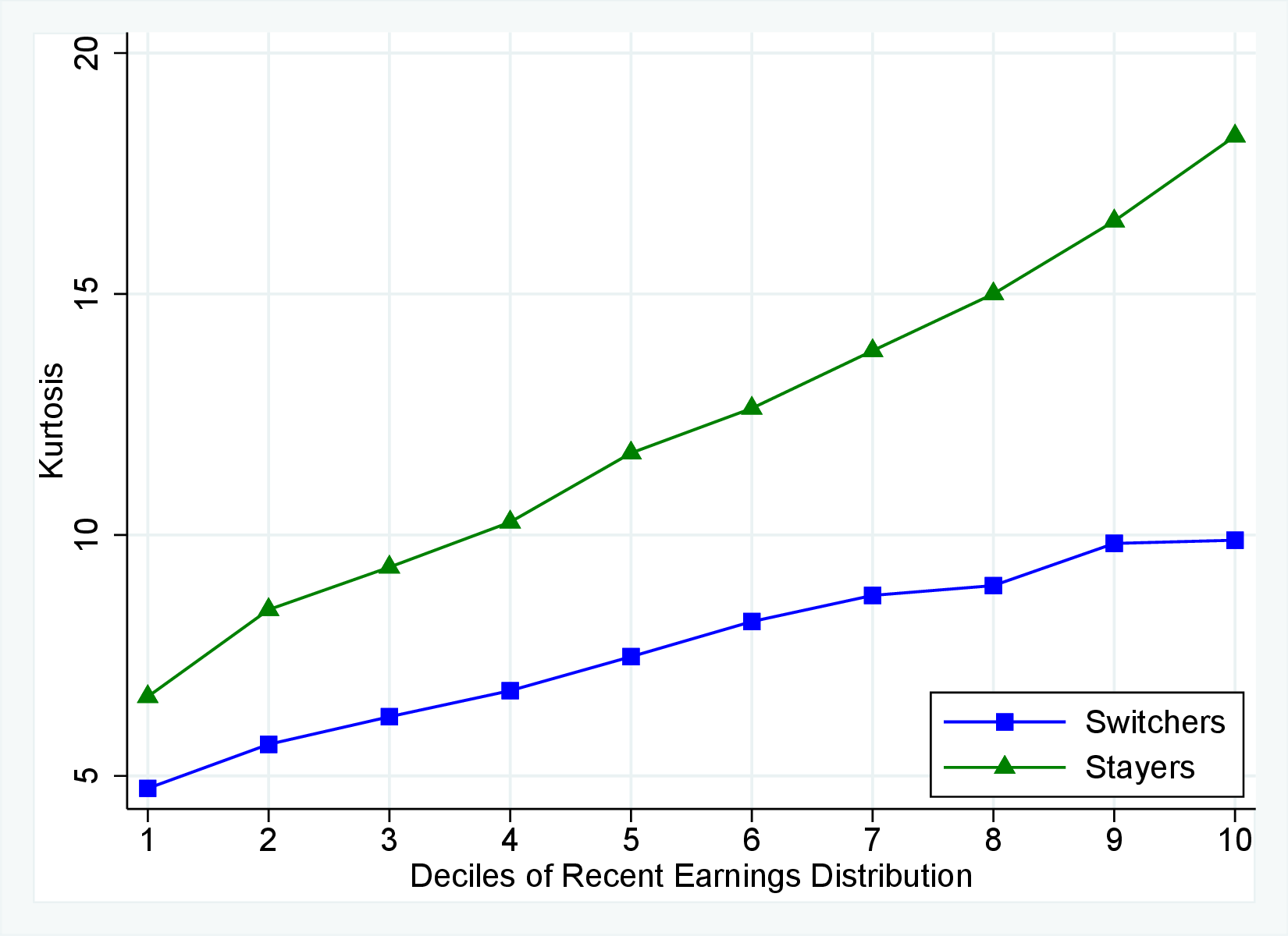
Figure: Figure E.7 – Kurtosis of Female Earnings Growth, Ages 25-55

11.4 Moments of Household Labor and Disposable Income Growth

Figure E.8 displays the variance of one-year and five-year income growth for the three income measures by income decile for females living as part of a couple. For females, the income of the spouse is an even more important insurance mechanism than it is for males. The insurance from the spouse is also more important than the tax and transfer system for one-year income growth.

In Figure E.9, we plot the skewness of one-year and five-year income growth of females living as part of a couple for the three income types by recent earnings decile. The pattern is the same as for men, with spousal income and the government both contributing to reducing the negative skewness.

Figure E.10 displays the kurtosis of one-year and five-year income growth of females living as part of a couple for the three income types by recent earnings decile. Adding the income from the spouse increases kurtosis for low-earning females and decreases it for high-earning females.

One-Year Growth

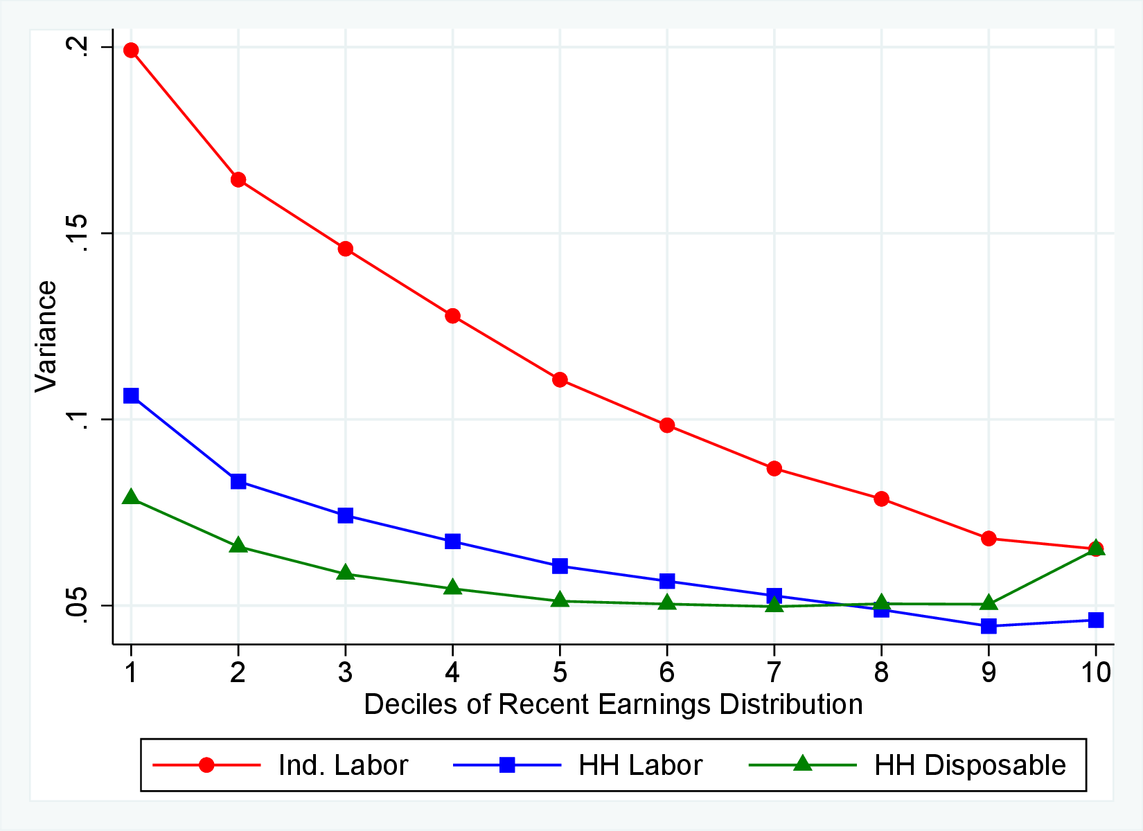
Five-Year Growth

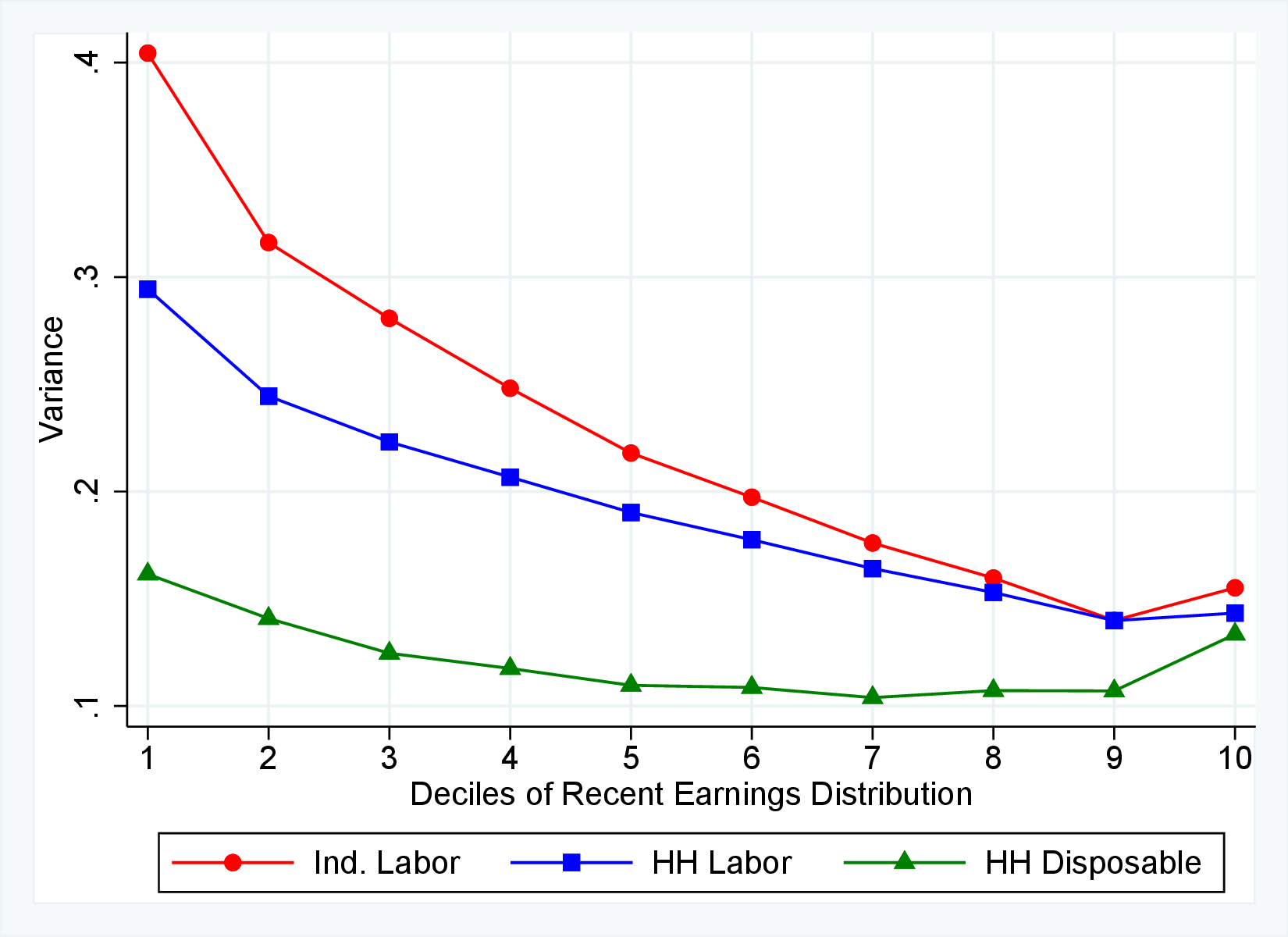
Figure E.8

–

Variance of the Growth of Different Income Measures (females in couple)

Note: The figure displays the variance of one-year (left) and five-year (right) log earnings changes (red line), log household earnings changes (blue line), and log disposable income changes (green line) for females of all ages (25-55), plotted for each decile of RE. The sample comprises married and cohabiting females and their households.

Figure: Figure E.8 – Variance of the Growth of Different Income Measures (females in couple)

One-Year Growth

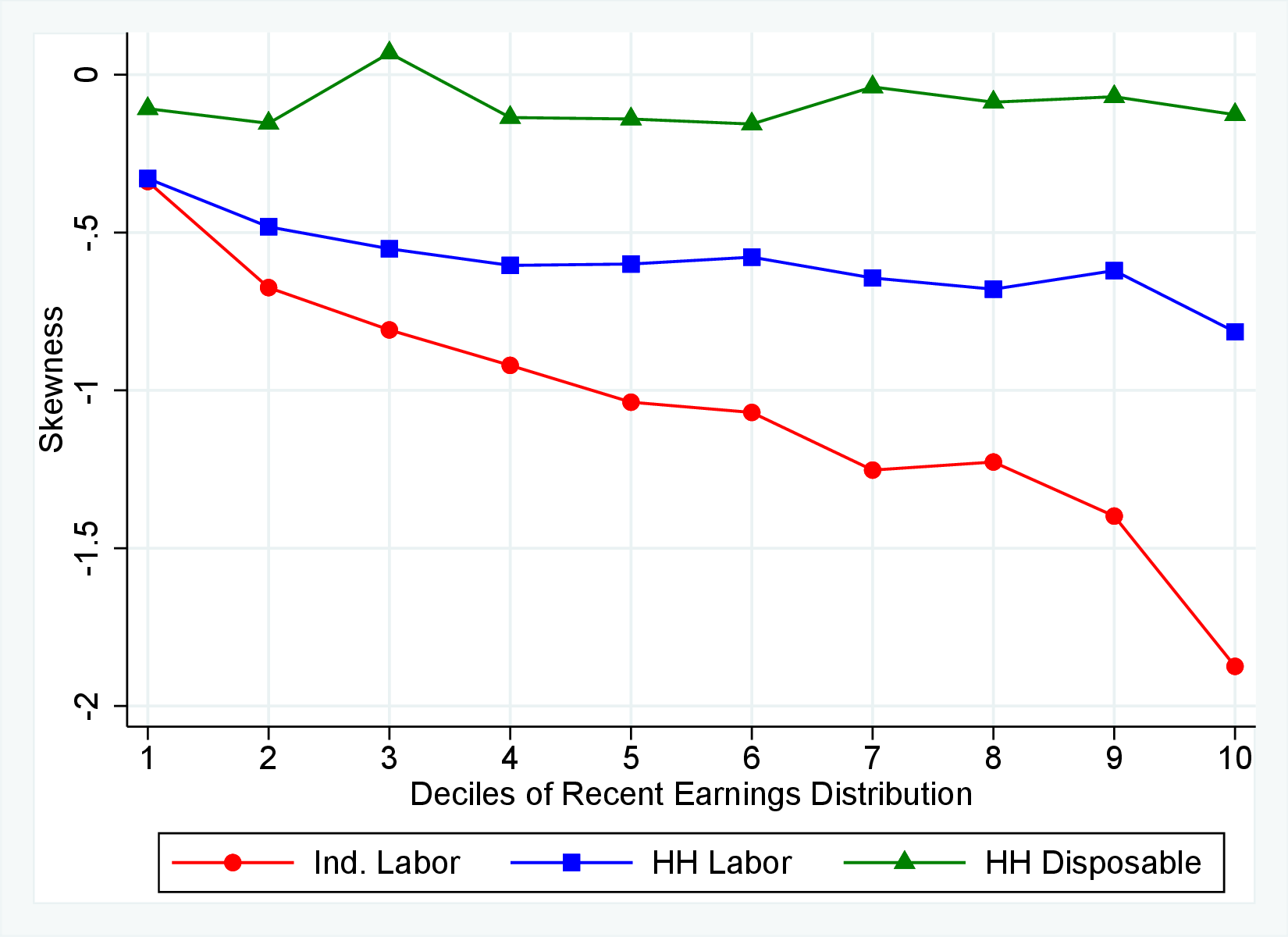
Five-Year Growth

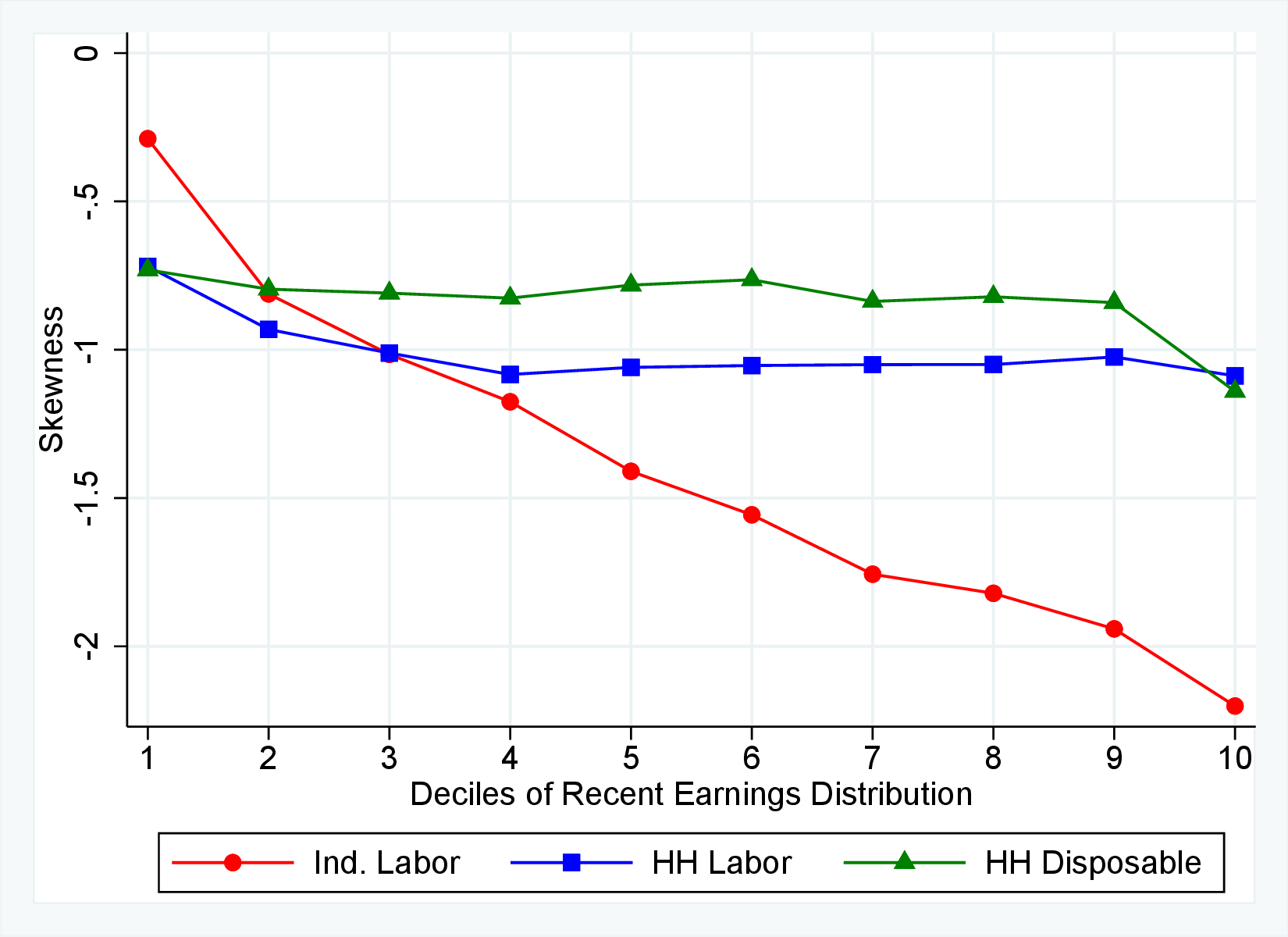
Figure E.9

–

Skewness of the Growth of Different Income Measures (females in couple)

Note: The figure displays the skewness of one-year (left) and five-year (right) log earnings changes (red line), log household earnings changes (blue line), and log disposable income changes (green line) for females of all ages (25-55), plotted for each decile of RE. The sample comprises married and cohabiting females and their households.

Figure: Figure E.9 – Skewness of the Growth of Different Income Measures (females in couple)

One-Year Growth

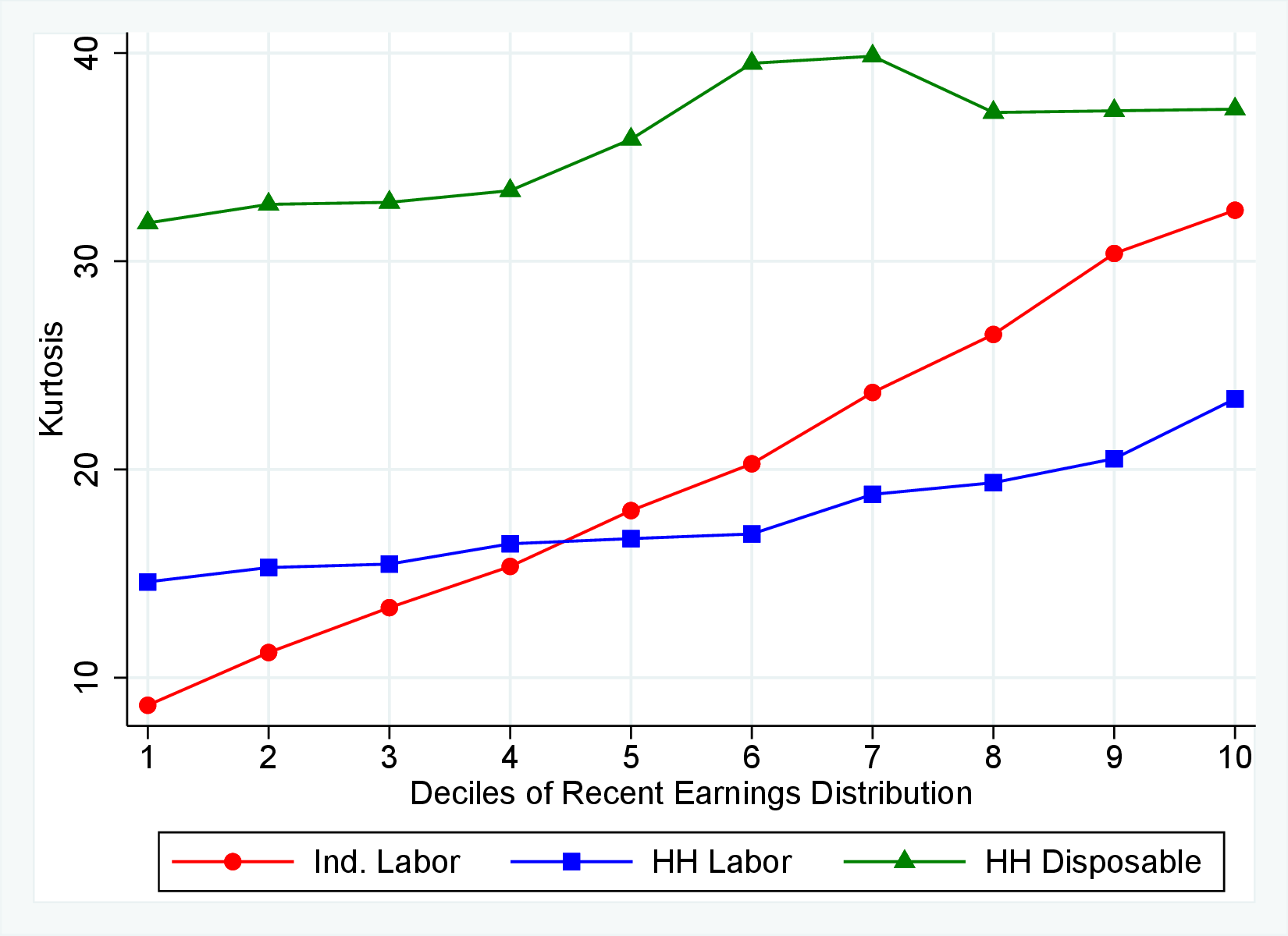
Five-Year Growth

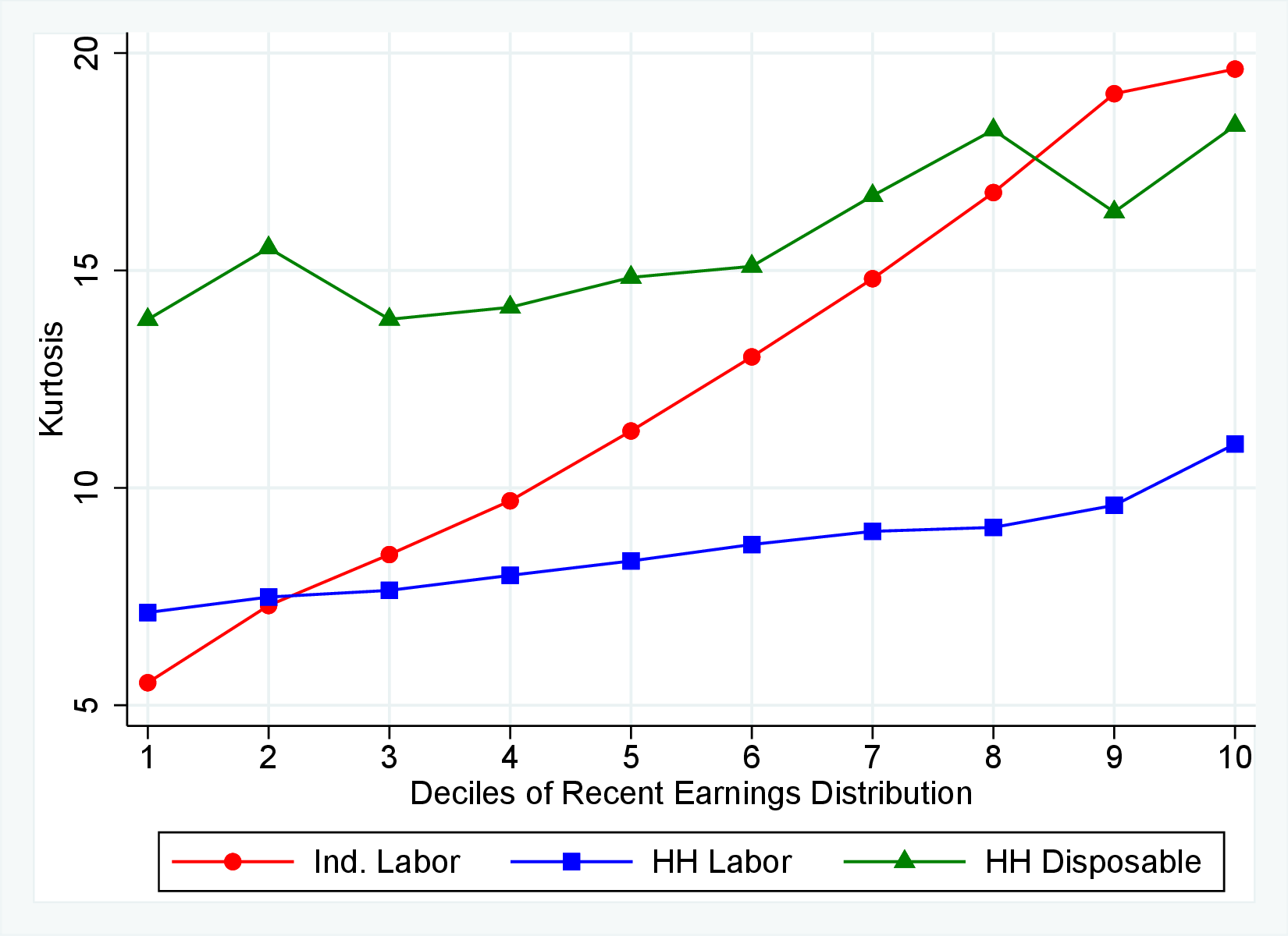
Figure E.10

–

Kurtosis of the Growth of Different Income Measures (females in couple)

Note: The figure displays the kurtosis of one-year (left) and five-year (right) log earnings changes (red line), log household earnings changes (blue line), and log disposable income changes (green line) for females of all ages (25-55), plotted for each decile of RE. The sample comprises married and cohabiting females and their households.

Figure: Figure E.10 – Kurtosis of the Growth of Different Income Measures (females in couple)

Footnotes

For example, if the asymmetric persistence and negative skewness of earnings changes were due entirely to changes in hours worked, then the policy prescriptions for taxation and social insurance might differ from what they would be if these features were instead driven by hourly wage growth.↩︎
We report the results for women in Appendix E, which show qualitatively similar patterns.↩︎
Their main (2001-2014) sample uses a measure of hours that does not include overtime for full-time workers (it is censored at full-time hours). The censoring is applied ex post by Statistics Netherlands to the uncensored measure of actual (rather than contractual) hours, which is available only before 2006 and used to validate their main results after 2006.↩︎
Among Norwegians, 5% have just business income but no labor earnings. An additional 5% have both labor earnings and business income, although for this group, business income tends to be small relative to labor income.↩︎
After 2014, a new system for reporting hours worked was introduced, leading to another major break in the data series. As a result, we only use data until 2014.↩︎
A survey week may therefore coincide with holidays as well as absence from work due to unemployment, sickness, or parental leave. Presuming that the probability of reporting is not affected by the work status, the random timing of the survey week will cause classical m.e. in hours worked but will otherwise not systematically affect our results. We return to this issue below.↩︎
For individuals who participate in the survey for only three quarters in year $t$, we impute annual hours as $h_{t,j}^{LFS}=(52/3)\cdot \sum _{j=1}^{3}h_{t,j}^{LFS}$, where $j$ represents the quarters for which the individual is sampled.↩︎
In general, we believe it is likely that surveys that intend to measure hours worked will be of a higher quality than administrative data on hours worked in settings where taxes and transfers are independent of hours worked (over and above earnings and employment status).↩︎
Heathcote et al. (2014) report a variance of log hours growth of 0.09 for working-age men in the PSID. Moreover, their estimate of classical m.e. implies a variance of m.e. in log hours growth of 0.072, implying that m.e. accounts for 80% of male hours growth.↩︎
We recognize that actual hours variable in AKU could contain m.e., which, as we argue below, is likely to be classical. It should, therefore, not cause a bias in Figure 1.↩︎
Quinlan (1992) developed the first version of this class of model tree algorithms as M5 algorithm.↩︎
We have also experimented with Poisson regression in the nodes, but this model did not outperform the linear regression model in terms of explanatory power and out-of-sample prediction.↩︎
Earnings contain valuable information which other variables do not capture. For example, it covaries with overtime, which neither of the other explanatory variables can capture. Excluding earnings as a regressor reduces the explanatory power of the imputation model and therefore leads to less precise measures of both hours and wage rates. This would, in turn, increase the variance of wage rate growth, lower the variance of hours growth, and lower the covariance between wage rate growth and hours growth, see Appendix A.4.↩︎
Information on part-time, full-time, sector of work, and change of employer is taken from the Employment Register. Education and marital status is taken from Administrative Tax and Income Records.↩︎
We have also experimented with alternative machine learning techniques and models, including LASSO, ridge regression, elastic net regression, neural network models, quantile regression, regression in growth instead of levels, allowing for more interaction between the explanatory variables, and other forms of more flexible parameterization. In the end, none of these alternatives outperformed the regression tree model in terms of explanatory power and out-of-sample prediction.↩︎
If earnings is dropped as an explanatory variable, the R-squared falls substantially for the PSID, whereas it remains high for the Norwegian register data. This can partially be explained by the availability of other independent variables on days receiving unemployment and sickness benefits.↩︎
The m.e. in AKU actual hours would be classical under the following three assumptions: (a) the week of survey is random; (b) the probability of responding to the survey is independent of whether the person is currently working or not; and (c) the distribution of m.e. is independent of observables such as earnings. Assumption (a) is true by construction. For (b) we note that it is mandatory to respond to the survey and non-response is in principle subject to a fine. The survey makes substantial effort to obtain answers, given that these data are the basis for the official employment and unemployment statistics. For example, AKU contacts each selected household up to 40 times before recoding them as a non-respondent. For (c) we observe that a simple statistic related to the level of m.e.—the covariance between wage rates and AKU hours—is similar across income groups. This suggests that the variance of m.e. in actual hours worked is similar across the earnings distribution.↩︎
However, the classical m.e. would still affect our results in Section 5 on higher-order moments of hours and wage growth, which we return to below.↩︎
Heathcote et al. (2010a) also restrict attention to individuals who work at least 200 hours per year. Guvenen et al. (2019) choose $Y_{\text{min},t}$ as the income from one quarter of full-time work at half of the legal minimum wage, which corresponds to 5% of median earnings in the U.S., but they have no information on hours worked. The constraint (iii) on hours curtails the sample by only 1% relative to constraints (i) and (ii).↩︎
The implication of this analysis is that RE percentiles are age group dependent. This ensures each RE group contains a similar number of observations. If we instead had grouped workers based on the RE distribution in the overall sample, too many younger workers would appear in lower RE percentiles and vice versa for middle-age workers. As a robustness check, we first group workers based on the RE distribution in the overall sample, and then within each RE group, we classify workers by age. We find that our main conclusions are robust to this change.↩︎
The individual log change $\Delta _{\log}^{k}z_{t}^{i}$ ignores some potentially valuable information on the extensive margin. For example, the long-term unemployed must be dropped (note that this caveat does not apply to the representative agent measure). Thus, for robustness we also conduct most of our individual-based analysis with an arc-percent change measure, $\Delta _{\operatorname{arc}}^{k}z_{t}^{i}=2(Z_{t+k}^{i}-Z_{t}^{i})/\left (Z_{t+k}^{i}+Z_{t}^{i}\right)$, which is not prone to this caveat and is commonly used in the firm dynamics literature. Our results are qualitatively robust to the choice of the individual-based growth rate measure. Results are available upon request.↩︎
Recall that workers are grouped into “young” (ages 25 to 35) and “prime age” (ages 36 to 55), and — within each age group — ranked into 10 deciles with respect to their recent earnings ($\bar{Y}_{t-1}^{i}$) in $t-1$.↩︎
The results when using the alternative measure of changes—the average of log earnings change within each group, $\Delta _{\log}^{k}z_{t}^{i}$—are qualitatively similar and are available upon request. We prefer to focus on the representative agent measures because this approach incorporates changes in the extensive margin of labor supply and does not require dropping observations close to zero.↩︎
While Jarosch (2021) investigates the scarring effects of unemployment on future employment, we consider the persistence of hours changes for all possible causes including sickness and changes in the intensive margin of labor hours. Moreover, different from Jarosch (2021), we study the heterogeneity in the persistence of hours changes for different income groups.↩︎
We group workers according to their one-year earnings changes instead of, e.g., five-year changes. Because, workers are more likely to experience multiple life cycle events over a five-year period, which would then weaken the links between earnings changes and particular events.↩︎
A weakness of this approach is that transitory shocks will be present—albeit less pronounced—even in five-year changes. An alternative approach would have been to model transitory and permanent changes following the methodology of Arellano et al. (2017). Future work should explore this approach for higher-order moments of persistent shocks.↩︎
For comparability, Figures B.1 and B.2 (from Guvenen et al. (2019)) and Figures B.3 and B.4 use same sample selection criteria. Specifically, the minimum hours threshold is not imposed in our sample.↩︎
Earnings changes for women are significantly less negatively skewed. For example, for women younger than 35, earnings changes are symmetric regardless of recent earnings.↩︎
Figure B.5 in Appendix B plots the percentile-based skewness measure, Kelly’s skewness, by RE and age, which displays similar patterns.↩︎
To see this, assume that the growth in log hours worked is measured with classical m.e., $\Delta \hat{h}_{i}=\Delta h_{i}+\epsilon _{i}$, and that wage rates are measured as earnings divided by hours. The growth in log wages therefore inherits the m.e. in hours: $\Delta \hat{w}_{i}=\Delta y_{i}-\Delta \hat{h}_{i}=\Delta w_{i}-\epsilon _{i}$. It follows that the covariance between observed hours growth and wage rate growth is biased downward by m.e.: $cov(\Delta \hat{h}_{i},\Delta \hat{w}_{i})=cov(\Delta h_{i},\Delta w_{i})-var(\epsilon _{i})$.↩︎
We focus on one-year earnings growth when analyzing stayers versus switchers since this approach allows for an unambiguous classification of switchers versus stayers.↩︎
Guvenen et al. (2019) impose a substantially more restrictive definition of a job stayer, namely, that the worker must have had some income in $t-1$ and $t+2$ from the same firm that was his main employer in periods $t$ and $t+1$. As a robustness check, we have applied their alternative definition of stayers. The results are qualitatively the same. Details are available upon request.↩︎
In this section, we calculate each moment controlling for year effects. Namely, we calculate moments for each year (for example, growth between 2008 and 2013) and take the average across years. Controlling for year effects has a negligible impact on the moments of labor income; however, it does matter when incorporating capital income. The reason is that a 2006 tax reform introduced a tax on dividends, increasing the maximum marginal tax on dividends from 28% to up to 48%. This reform was announced in advance, and owners took out substantial dividends in 2005. Aggregate dividends as a share of aggregate GDP increased by 47% from 2004 to 2005 and fell by 93% from 2005 to 2006. Excluding or including data for the years 2005 and 2006 has an impact on the moments if data are pooled but has negligible effects when controlling for year effects.↩︎
A more detailed analysis shows that the progressive tax system also contributes to lowering the variance, especially for men above the median. However, the main driver of the big reduction in the variance of income growth relative to earnings growth is the generous transfer system.↩︎
They also calculate individual disposable labor income and find that the variances of shocks to individual disposable income are just slightly larger than those of household disposable labor income.↩︎
Recall bias is a systematic error that occurs when participants do not accurately remember previous events.↩︎
We use a Python implementation of this algorithm by Anson Wong: https://github.com/ankonzoid/LearningX/tree/master/advanced_ML/model_tree↩︎
We have also experimented with Poisson regression in the nodes but this model did not outperform the regression tree model in terms of explanatory power and out-of-sample prediction.↩︎
When excluding earnings as an explanatory variable for hours, some of the true variation in hours that is captured by earnings (and which is not captured by the non-earnings regressors) get subsumed in hourly wages instead of being attributed to hours. This introduces m.e. in both hours and wage rates. For example, the variance of five-year wage rate growth increases by about 0.03 and the variance of five-year hours growth declines by almost 0.01 when excluding earnings from the hours imputation. Moreover, the covariance between these variables declines by 0.017 when earnings is excluded as a regressor relative to the case when earnings is included in the imputation. This suggests that m.e. in imputed hours is substantially smaller when earnings is included as a regressor. We conclude that not including earnings as a regressor would give a too high weight to wage rates in accounting for earnings shocks.↩︎
Arc percent change of variable $x$ between $t$ and $t+1$ is given as $2(x_{t+1}-x_{t})/(x_{t+1}+x_{t})$, which allows for low values in either year (in contrast to the log growth measure).↩︎
Note that the relevant R-square for the hours imputation is that of the out-of-sample prediction reported in Table I. The R-squared in Tables A.3-A.4 refer to the predictive power of the linear regressions at the terminal nodes of the regression tree, i.e., after going down the branches of the regression tree.↩︎
We have also experimented with Poisson regression in the nodes, but this model did not outperform the regression tree model in terms of explanatory power and out-of-sample prediction.↩︎